IT Literature Intelligence 终审版本 (VERIFIED) 论文编号: 195 | 原始基线: V0_ZCODE_BASELINE | 语义审核: pass | 图表审核: pass

Learning view invariant recognition with partially occluded objects

Tromans · Frontiers in Computational Neuroscience · 2012 · Zotero itemID=1815

一句话定位：这篇论文回答了一个很"接地气"的问题——当某个物体在训练中始终被别的物体部分遮挡时，视觉系统还能不能为它建立一个跨视角不变（view invariant）的表征？作者用腹侧视觉通路的神经网络模型 VisNet 模拟六个 3D 物体一起旋转（中央的 Jaimoid 永远被五个遮挡物部分遮住），首次证明仅靠标准 Hebb 规则的连续变换学习（CT learning）就能把被遮挡物体的各个"部分视图"绑成一个整体不变表征。这是 Stringer 等人此前只停留在假说层面的想法第一次得到模拟证据，对理解真实场景中的无监督物体学习很有价值。

研究背景

灵长类视觉系统在逐级加工中形成对物体具有视角、尺寸、位置（平移）不变性的神经元响应，这在下颞叶皮层（inferior temporal cortex, IT）已有充分证据（如 Booth & Rolls 1998 的视角不变细胞、Tovee 等 1994 的平移不变面孔细胞）。但在自然场景里物体很少单独出现：已有工作表明，VisNet 可以在训练时多个物体同时存在、甚至没有任何一个物体被单独见过的情况下，靠"物体内特征共现频率远高于物体间特征共现"的统计独立性，学会分别表征各个物体（Stringer et al., 2007; Stringer & Rolls, 2008）；也可以识别放在自然杂乱背景上、此前单独学过的物体（Stringer & Rolls, 2000），但若训练时物体本身就摆在杂乱背景上则学习失败。

真正的缺口在于遮挡：自然环境中物体经常互相重叠，一个物体在训练中可能总是被部分遮挡。这时网络面临双重任务——既要把被遮挡物与遮挡物分开，又要把同一物体在不同时刻露出的不同"部分视图"连接成一个完整的不变表征。Stringer 等（2007）曾提出连续变换学习（Continuous Transformation, CT learning）结合物体组合的统计独立性或许能解决此问题，但没有给出任何模拟证据。本文的目的就是补上这个证据，并且用的是带光照、按 1° 步长连续旋转的真实感 3D 物体，比以往 2D 平移实验更接近真实视觉。

研究思路

作者的总逻辑是两条机制的接力。第一条是统计独立性：训练时物体以不同的配对组合出现（Jaimoid 依次与五个遮挡物配对，五个遮挡物之间也两两配对旋转），使得同一物体内部的特征总是同时出现、完全相关，而任意两个物体之间的特征只偶尔共现——竞争网络于是会把"高频共现的特征集合"分配给输出神经元，形成单个物体的表征而非"场景组合"的表征。第二条是 CT 学习：同一物体相继视角之间存在空间相似性（部分输入滤波器保持激活），Hebb 联想学习会在物体连续变换时让同一个输出细胞不断"接管"新的输入连接，最终该细胞对物体的所有（或绝大多数）视角响应——不需要时间痕迹，只用最简单的 Hebb 规则，生物合理性反而更高。

作者明确对比了两种不变性学习机制的分工：CT 学习利用视角间的空间相似性，trace 学习（Földiák 1991）利用变换在时间上的连续性；本文只测试 CT 学习。被遮挡物体是难点所在：它从未以完整面貌出现，网络必须把训练中先后露出的不同碎片视图连接起来。作者用三类测试来验证结果不是假象——单独旋转测试（不变性）、新物体同位置测试（排除"学到的是位置而非物体"）、碎片部分视图测试（排除"依赖某个关键标记 key-marker"）。

方法

模型为 VisNet：四层各 32×32 神经元的层级竞争网络，依次对应 V2、V4、后下颞皮层与前下颞皮层；前馈连接来自前一层拓扑对应区域、按高斯分布采样（Table 1：各层会聚半径 6/6/9/12，连接数 272/100/100/100，视网膜输入 128×128×32）。输入用模拟 V1 简单细胞的 DOG（difference of Gaussians）滤波器组，调谐于空间频率（0.0625–0.5 周期/像素，4 个倍频程）、取向（0°–135°，步长 45°）与符号（±1）（Table 2 给出各频率组的连接数）。层内竞争分两步：先用空间滤波器做侧抑制（Table 3：σ = 1.38/2.7/4.0/6.0，δ = 1.5/1.5/1.6/1.4），再用 sigmoid 做对比增强并按每层百分位阈值控制发放稀疏度（Table 4：百分位 95/95/88/91，斜率 β = 190/40/75/26）。学习规则为标准 Hebb 规则 δwij = α·yi·xj，每个时间步末做权重向量归一化以防少数神经元垄断。

刺激为 6 个 Swift 3D 5.4 建模的 3D 物体（环境光加单漫射光源），每个绕竖直轴以 1° 步长旋转 360°、导出 360 帧 2D 图像。五个遮挡物为锥体（cone）、立方体（cube）、圆柱（cylinder）、星形（star）、十二面体（dodecahedron），被遮挡物为不规则多面体 Jaimoid。空间布局为五边形阵（图 3）：Jaimoid 居中、五个遮挡物在五个顶点处与它部分重叠且等距，保证遮挡程度可比。修改为：“训练序列包含 Jaimoid 与 5 个遮挡物分别配对的 5 段序列，以及 5 个遮挡物所有可能的成对组合（10 段），总计 15 段（每段 360 帧）”或直接删去“共五段”。（同时演示遮挡物之间的互相遮挡）；逐层训练 50 个 epoch，学习率第 1 层 0.109、其余层 0.1。由于计算开销大，只有 Jaimoid 被部分遮挡。测试时权重固定：单独旋转测试、六个新物体（tee、torus、hectoid、irinoid、church、pyramid）同位置测试、以及碎片部分视图测试；性能用单细胞信息 I(s,R) 与多细胞信息 I(S,S′)（经 Bayes 解码，取每个物体信息最高的前 5 个细胞、共 30 个）量化，六个物体的理论上限为 log2 6 ≈ 2.58 bits。

主要结果

训练后出现"排他性不变细胞"：第 4 层随机选中的细胞 (4,17) 训练前对六个物体随机响应，训练后只对中央被遮挡的 Jaimoid 在所有（或至少 80%）视角响应、对其他物体任何视角都不响应（图 12）；细胞 (19,1) 则对十二面体的全部 360 个视角不变响应（图 13）。六个物体各由一组独特的输出细胞单独表征。
不变性沿层级递增：对 Jaimoid 响应的各层示例细胞中，第 3 层已高度变换不变且物体特异，第 2 层不变性较温和，第 1 层几乎不变性、只响应很窄的视角范围（图 14）——与"会聚逐层累积不变性"的架构假设一致。提高稀疏度会使表征更分布式（排他细胞减少、物体身份由细胞群编码），结果对该参数稳健。
碎片视图被绑成整体：用训练中从未以完整形式出现过的碎片部分视图单独测试时，细胞 (4,17) 对每个碎片视图的响应方式与看完整 Jaimoid 时完全一致（图 15）——证明识别不依赖任何关键标记或特定部分视图，网络确实把各部分视图绑成了一个整体不变表征。
学到的是物体而非位置：尽管训练与测试中物体位置高度重叠，输出细胞仍只对物体身份响应；换成六个新物体放在与训练集完全相同的位置上，细胞 (4,17) 与 (19,1) 都只对少数物体的少数视角有微弱响应、不再有不变响应（图 16、17），单细胞信息也没有细胞达到最大值。
信息论确认：单细胞信息显示大量第 4 层神经元对训练物体达到最大值 2.58 bits（随机未训练网络为基线，图 18）；多细胞信息训练后超过 2.5 bits，远高于未训练网络的 1.10 bits 与训练网络测新物体时的 1.7 bits（图 19）——六个物体全部被独立编码，且编码的不是位置。

图注解读

图 1 · CT 学习的单层示意

原文图注：FIGURE 1 | An illustration of how CT learning functions in a feed-forward one-layer network. Activation of overlapping neurons during the transformation of the object from position to position leads to the activation of the same neuron in the output layer. Connections are strengthened according to a Hebbian learning rule after each presentation of the stimulus.

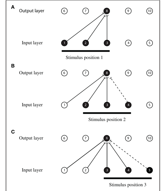
解读：三步示意图：刺激在位置 1 时输入层 1/2/3 号神经元激活，输出层 8 号细胞经随机连接胜出并被 Hebb 规则增强；刺激移到位置 2（输入变为 2/3/4，与之前重叠两个单元）时，已增强的连接让同一个输出细胞再次胜出，新输入连接随之被加强。反复下去，同一输出细胞就学会了响应不断变换中的同一物体——这是全文方法的核心直觉。

图 2 · 六个训练物体

原文图注：FIGURE 2 | The six objects used to train the network. The objects are 3D objects each shown from 360 different views. The effect of the ambient lighting and single diffuse light source is illustrated. This allows different surfaces to be shown with different intensities. Objects are split into two groups; occluding objects are presented in the top row and the occluded object is presented in the bottom row.

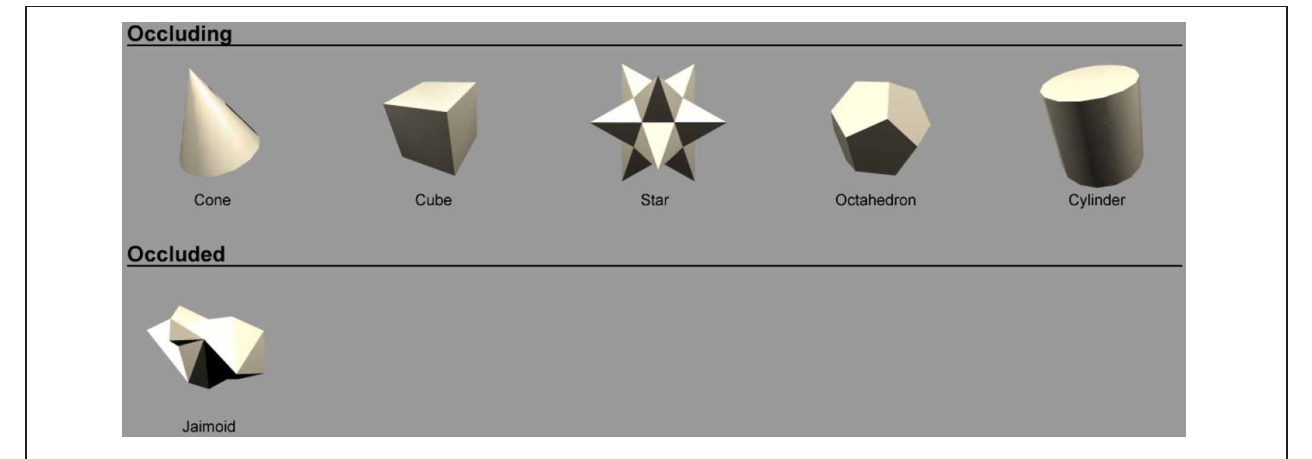
解读：训练刺激一览：上排五个遮挡物、下排被遮挡的 Jaimoid，均为 3D 渲染物体（各 360 个视角），环境光加单漫射光源使不同表面呈现不同亮度。这张图交代了刺激的"真实感"来源——有光照、有明暗面，比此前的 2D 线条图形更接近自然视觉。

图 3 · 五边形布阵示意

原文图注：FIGURE 3 | The pentagon formation specifying the location of the occluding and occluded objects. The occluded object, the Jaimoid, is always presented in the centre of the pentagon. Each of the occluding objects is placed at one of the five points of the pentagon, partially overlapping the Jaimoid at the center. This ensures that the occluding objects are equidistant from the center of the occluded object, helping to maintain a comparable level of partial occlusion for the Jaimoid.

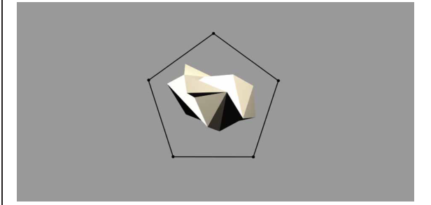
解读：布阵规则图：Jaimoid 恒居五边形中心，五个遮挡物各占一个顶点、与 Jaimoid 部分重叠且到中心等距。这样设计是为了让不同遮挡物对 Jaimoid 的遮挡程度可比——把"遮挡量"这一混杂变量固定下来，后面结果才能干净地归因于物体身份。

图 4 · Jaimoid 单独旋转的测试序列

原文图注：FIGURE 4 | Five example frames selected from the 360 frame testing image sequence of the Jaimoid rotating in depth around the vertical axis through 360° in 1° steps. The selected frames shown are for 0°, 72°, 144°, 218°, and 288°.

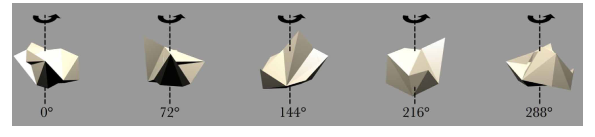
解读：测试时单独呈现 Jaimoid 的 360 帧序列中的五个示例帧（0°、72°、144°、218°、288°）。这张图定义了"完整视角测试"的刺激形态，也直观展示这个不规则多面体在不同深度旋转视角下的外观差异。

图 5 · VisNet 四层架构与脑区对应

原文图注：FIGURE 5 | Left: Stylised image of the 4 layer network developed by Wallis et al. (1993) and Wallis and Rolls (1997). Convergence through the network is designed to provide fourth layer neurons with information from across the entire input retina. Right: Convergence in the visual system V1, visual cortex area V1, TEO, posterior inferior temporal cortex; TE, inferior temporal cortex (IT).

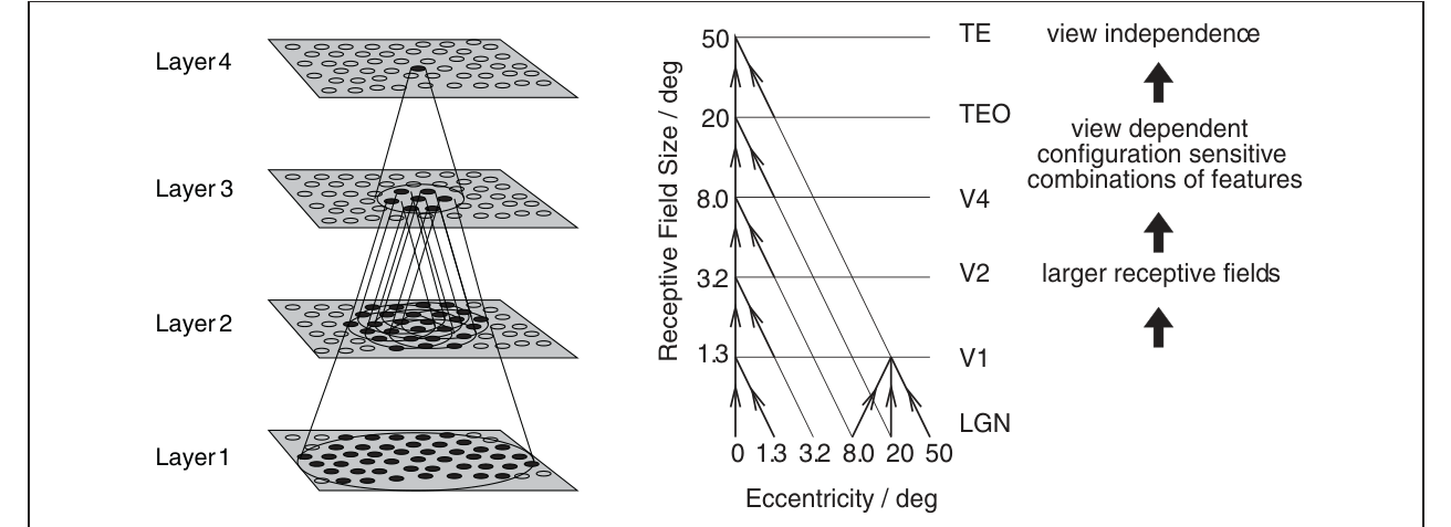
解读：左图为 VisNet 四层网络的程式化示意，右图为脑中 V1→V2→V4→TEO→TE 的逐级会聚及感受野随偏心距扩大的数据（1.3°/3.2°/8.0°/20°/50° 量级）。作者用这张图把模型层与脑区一一对应，说明"会聚导致感受野逐层扩大"既是生物学事实也是模型设计原则。

图 6 · 输入滤波器采样范式

原文图注：FIGURE 6 | The filter sampling paradigm. Images are first filtered by a difference of Gaussian filter of the appropriate orientation, sign, and frequency. Each square represents the retinal image after filtering and the circles represent the consistent retinotopic coordinates used to provide input to a layer one cell. The orientation tuning, left to right, increases from 0° in steps of 45°, with segregated pairs of positive (P) and negative (N) filter responses. The filters double in spatial frequency toward the reader. For further details, see Rolls and Deco (2002).

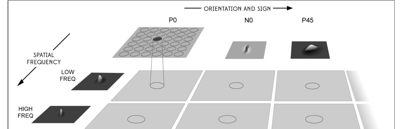
解读：与 Rolls 综述中的同名图呼应：每个方格是经某 DOG 滤波器（列按取向、行按空间频率，P/N 正负输出分开）处理后的视网膜图像，圆圈标出第 1 层细胞的一致视网膜拓扑采样坐标。它说明网络的"V1 输入"如何从图像中提取取向与频率信息。

图 7 · Jaimoid 与锥体成对旋转的训练序列

原文图注：FIGURE 7 | Five example frames selected from the 360 frame training image sequence of the Jaimoid and the Cone rotating through 360° in 1° steps. The selected frames shown are for 0°, 72°, 144°, 218°, and 288°. All five of the occluding objects were also presented to the network in the same manner.

解读：训练序列示例：Jaimoid 与锥体成对、各自绕自己的竖直轴同速旋转的五个帧。五段训练序列都是这个形式，只是配对物换成其余四个遮挡物。两物体绕平行轴同步旋转，正是"被遮挡物从未单独出现"这一训练条件的呈现方式。

图 8 · 五个遮挡物各就各位

原文图注：FIGURE 8 | Five example frames of the Jaimoid occluded by all five occluding objects in their five corresponding positions. The occluding objects are arranged around the pentagon formation so that they are equidistant from the center of the Jaimoid. The rotating objects used during training are presented in the same locations: cone, position 1; cube, position 2; cylinder, position 3; star, position 4; dodecahedron, position 5; Jaimoid, position 6.

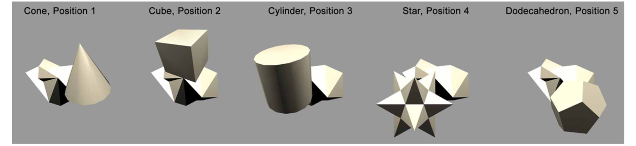
解读：五个示例帧展示五个遮挡物按五边形顶点位置（锥、立方体、圆柱、星、十二面体依次在位置 1–5，Jaimoid 在中心位置 6）排布时的整体场景。它给出各物体的空间"户口"——所有物体在训练和测试中都占据这些高度重叠的固定位置，这正是第 3.4 节"位置 vs 物体"检验的实验前提。

图 9 · 遮挡物之间的互相遮挡

原文图注：FIGURE 9 | Five example frames of two occluding stimuli (cylinder and star) rotating together, demostrating the typical overlap between the occluding objects.

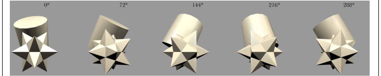
解读：圆柱与星形两个遮挡物成对旋转的五帧示例，展示遮挡物彼此之间也常有重叠（相邻对会互相部分遮挡）。这说明训练集里不止 Jaimoid 一个"受害者"——统计独立性机制需要应付的正是这种多重重叠。

图 10 · 五对物体的互遮挡部分视图

原文图注：FIGURE 10 | Mutual overlap: Areas of mutual overlap between the occluding and occluded objects during one example frame of rotation. As the two objects rotate together in lock-step, the area of mutual overlap creates a partial view of the occluded object: (A) Shows the cone and Jaimoid; (B) Cube and Jaimoid; (C) Cylinder and Jaimoid; (D) Star and Jaimoid; (E) Dodecahedron and Jaimoid. Each pair is presented alongside the partial view it creates. VisNet must learn to associate together all of these different partial views of the occluded object to build an exclusively invariant representation.

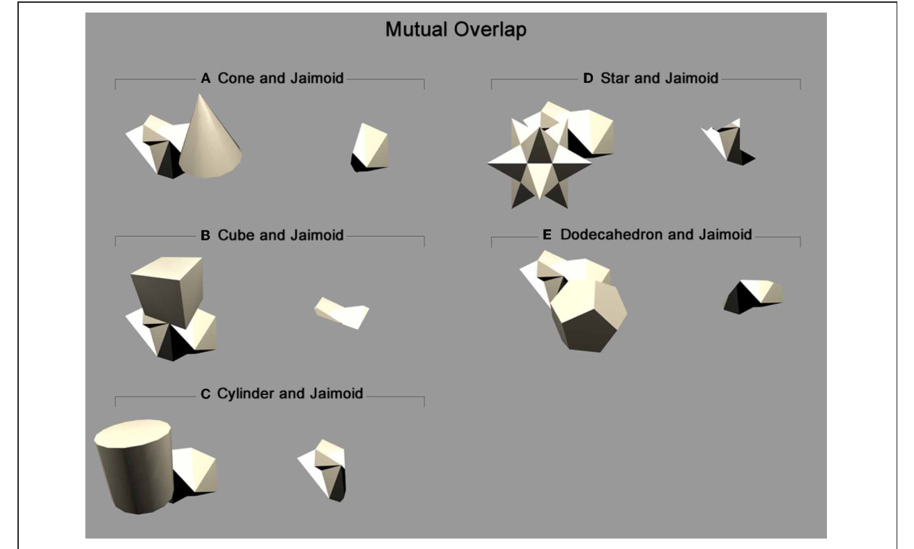
解读：五组"配对帧 + 其产生的部分视图"：Jaimoid 分别被锥体、立方体、圆柱、星形、十二面体遮挡时露出的部分各不相同。这张图把问题可视化——Jaimoid 在整个训练中从未完整露面，网络见到的只是这些不断变化的碎片，它必须把五组碎片全部连成一个不变表征。

图 11 · 星形与 Jaimoid 的互遮挡细节

原文图注：FIGURE 11 | Star and Jaimoid mutual overlap: Five example frames of the star and Jaimoid as they rotate together in lock-step. As in Figure 10, the area of mutual overlap creates a partial view of the Jaimoid. This is shown in this specific example where the star and Jaimoid are presented over five equally spaced viewing angles.

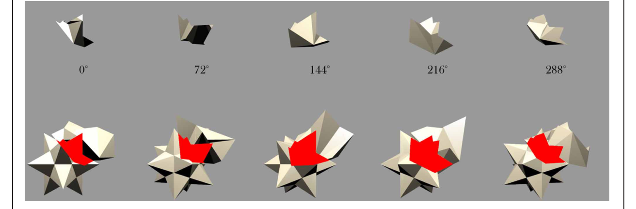
解读：图 10 的局部放大：星形与 Jaimoid 同步旋转经过五个等间隔视角时，互遮挡区域形成的 Jaimoid 部分视图随之变化。随视角连续变化的部分视图正是 CT 学习赖以工作的"空间相似性链"——相邻视角间的重叠输入是学习的接续点。

图 12 · 细胞 (4,17) 训练前后对六个物体的响应

原文图注：FIGURE 12 | The firing rate responses of cell (4, 17) in the 4th (output) layer of VisNet to the central occluded object (Jaimoid) and the five surrounding occluding objects as they rotated through 360° in 1° steps before and after training. Before training, it can be seen that the cell responds randomly to different views of different objects. After training, it can be seen that the cell's response pattern has changed. This cell responds to all the views of Jaimoid, and to none of the views of the other objects.

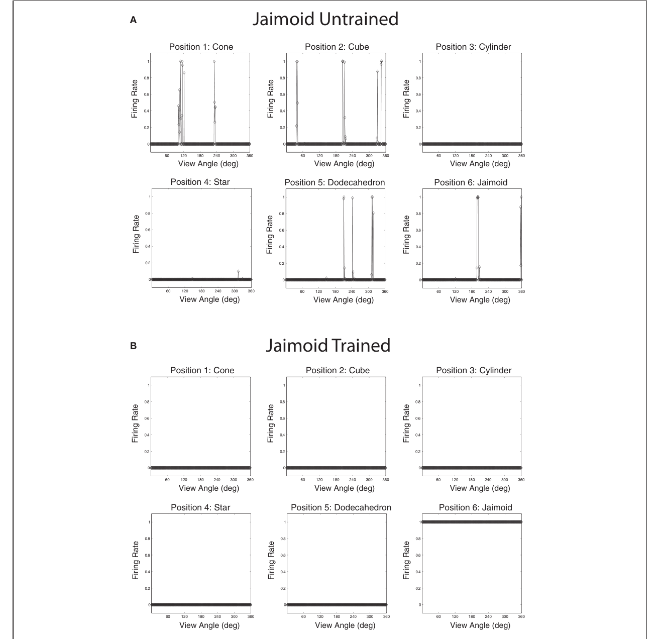
解读：12 张小图（训练前 A、训练后 B 各六张），每张为该细胞对一个物体 360 个视角的放电率曲线。训练前六条曲线杂乱无章；训练后只有 Jaimoid 的曲线在整个 0–360° 范围内持续高放电，其余五个物体全为零。这是"被遮挡物获得了视角不变表征"最直接的单细胞证据，也是图 15 碎片视图测试的参照系。

图 13 · 细胞 (19,1) 成为十二面体的排他不变细胞

原文图注：FIGURE 13 | The firing rate responses of cell (19, 1) in the fourth (output) layer of VisNet to the central occluded object (Jaimoid) and the five surrounding occluding objects as they rotated through 360° in 1° steps before and after training. Before training it can be seen that the cell responds randomly to different views of different objects. After training it can be seen that the cell's response pattern has changed. This cell has become an exclusive invariant cell for the Dodecahedron. It responds invariantly to all 360 views of the Dodecahedron and to no views of any other object.

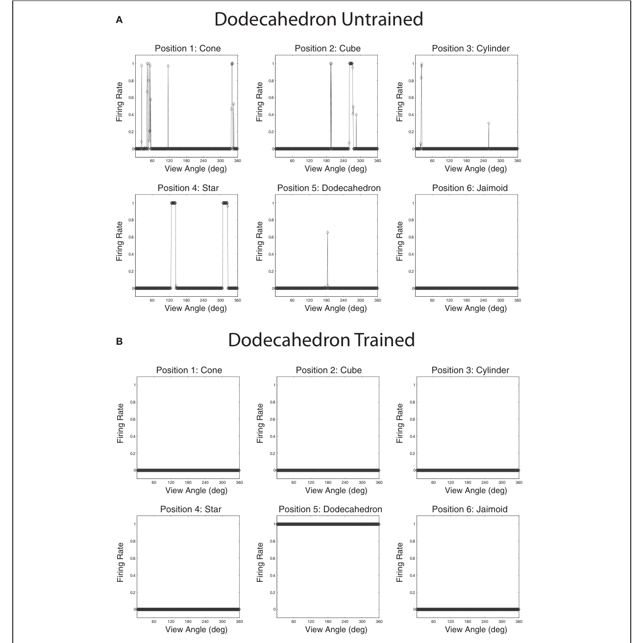
解读：与图 12 同构，但主角换成细胞 (19,1)：训练后它对所有 360 个视角的十二面体不变响应、对其余物体（包括 Jaimoid）无任何响应。这说明遮挡物本身虽然总是与 Jaimoid 重叠出现，也各自被单独表征——"分离物体"这一半任务同样完成。

图 14 · 四个层级对 Jaimoid 的响应对比

原文图注：FIGURE 14 | Example Jaimoid response plots for all four layers. A prototypical example cell is presented for each of the 4 layers within the VisNet model. For each cell, its response plot is presented with respect to the example object, the Jaimoid. It can be seen that a typical layer 3 cell is highly transform invariant while a layer 2 cell shows more modest levels of view invariance. Layer 1 cells demonstrate very little view invariance and responded to a very narrow set of views. In all cases, these cells responded exclusively to their preferred object, in this case the Jaimoid, and did not learn to respond to any views of any of the other objects. Comparable responses exist for all six of the objects presented during training.

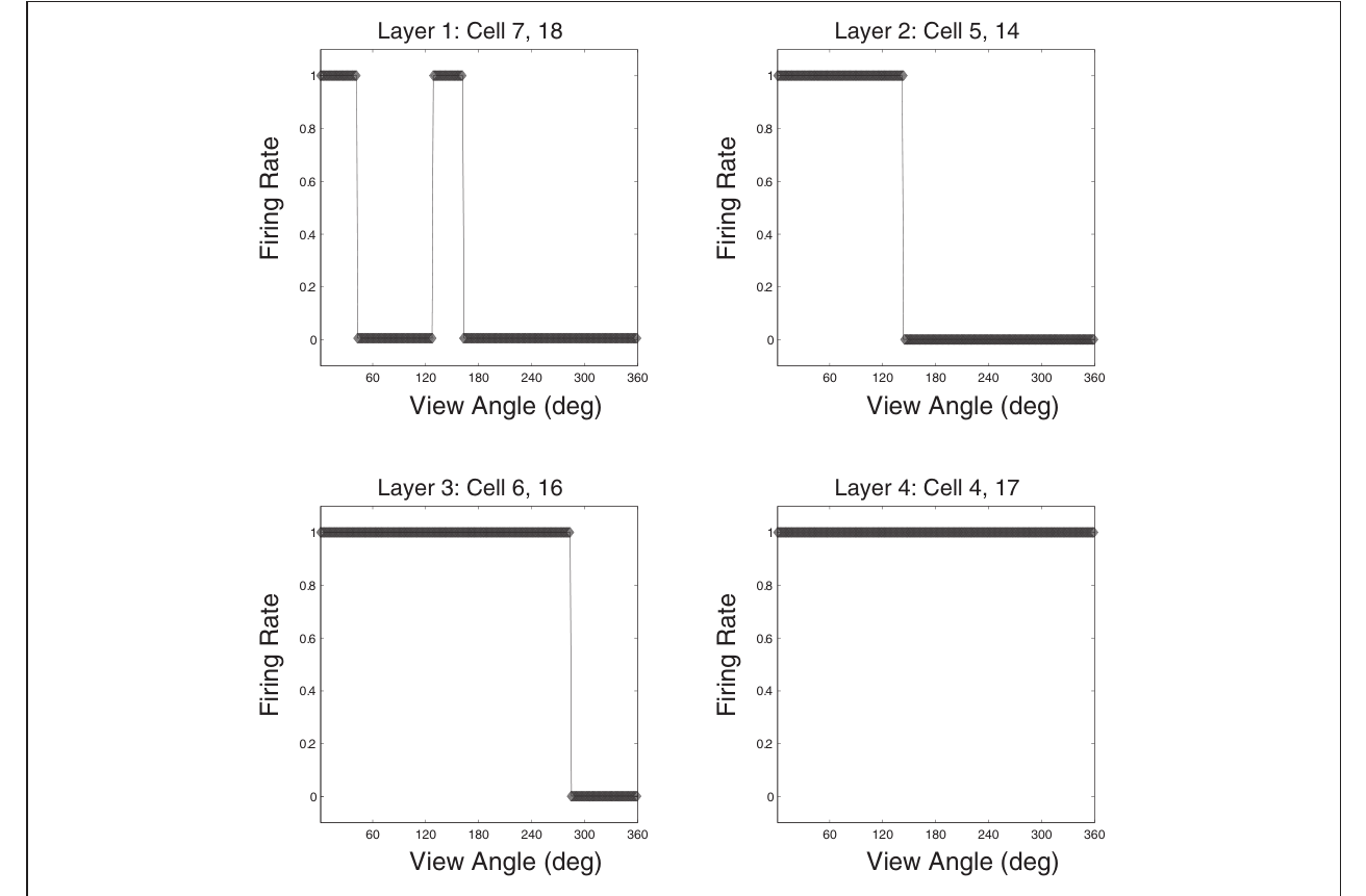
解读：四个层级各取一个对 Jaimoid 响应的典型细胞：第 1 层只在很窄的视角段响应、第 2 层不变性温和、第 3 层已高度不变、第 4 层满覆盖（另有物体特异性）。这张图把"不变性逐层累积"的过程拆开给人看，对应 Rolls 综述中判别因子逐层递增的现象。

图 15 · 碎片部分视图测试

原文图注：FIGURE 15 | Partial view response plots for cell 4, 17. Cell response plots are presented after testing the network with the fragmented partial views of the Jaimoid, as exemplified in Figure 10. It can be seen that the example cell 4, 17 that responded invariantly to the complete view of the Jaimoid also responds in an identical manner to the different fragmented partial views of the Jaimoid. Cell 4, 17 has learned to bind together these different partial views into a holistic representation and responds equally well to all of them, thus proving that this cell does not rely on a specific partial view or key-marker in order to recognize the Jaimoid.

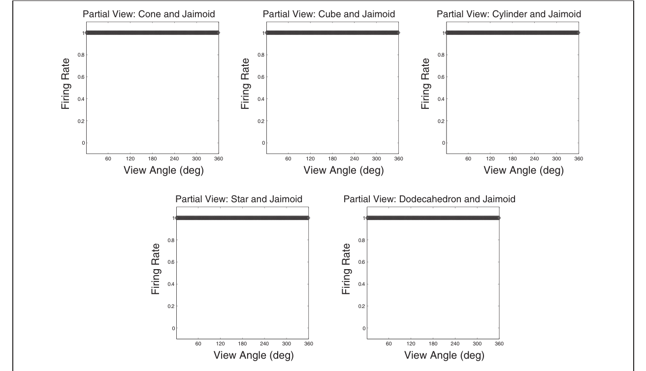
解读：五张小图对应五种遮挡条件下产生的 Jaimoid 碎片视图序列，细胞 (4,17) 对每一个碎片视图的响应都与看完整 Jaimoid 时一致。这张图是全文最关键的新颖结果：识别不是靠某个恒定露出的"关键标记"（否则换一种遮挡方式响应就该消失），而是把所有部分视图真正绑成了一个整体表征。

图 16 · 细胞 (4,17) 对六个新物体的响应

原文图注：FIGURE 16 | The firing rate responses of cell (4, 17) in the fourth (output) layer of VisNet to six new objects that the network was not trained on, as they rotated through 360° in 1° steps after training. It can be seen that the cell's response pattern has changed compared to its response pattern to the six objects that the network was trained on (the occluded and the five occluding objects; Figure 12B). Whereas when tested with the set of objects that the network was trained on, the cell responds to at least 80% of the views of Jaimoid, and to none of the views of the other objects. When the network is tested on six novel objects presented in the same locations as the trained set of objects, the cell responds very poorly to small portions of view of a number of objects. This shows that the network has learnt to respond to the trained objects in particular, and not just to their locations.

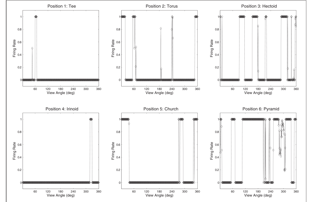
解读：六个新物体（tee、torus、hectoid、irinoid、church、pyramid）摆在训练集的相同位置上旋转，细胞 (4,17) 只对其中若干物体的少数视角有微弱放电、没有任何不变响应。与图 12B 对照（对 Jaimoid 至少 80% 视角响应），这排除了"细胞只是记住了位置"的备择解释——它学的是训练物体的视觉形态本身。

图 17 · 细胞 (19,1) 对六个新物体的响应

原文图注：FIGURE 17 | The firing rate responses of cell (19, 1) in the fourth (output) layer of VisNet to six new objects that the network was not trained on, as they rotated through 360° in 1° steps after training. It can be seen that the cell's response pattern has changed compared to its response pattern to the six objects that the network was trained on (the occluded and the five occluding objects; Figure 13B). Whereas when tested with the set of objects that the network was trained on, the cell responds invariantly to all 360 views of the Dodecahedron and to no views of any other object. When tested on the six novel objects presented in the same locations as the trained set of objects, the cell responds very poorly to small portions of view of a number of objects. This shows that the network has learnt to respond to the trained objects in particular and not just to their locations.

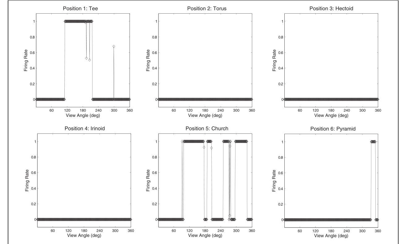
解读：与图 16 平行的对照，主角为十二面体的排他细胞 (19,1)：面对同位置的新物体同样只有零星微弱响应。两个代表性细胞都通过"新物体测试"，物体选择性而非位置选择性的结论因此有双重证据。

图 18 · 单细胞信息分析

原文图注：FIGURE 18 | Single cell information results obtained when VisNet was tested with the occluded object and five occluding objects rotating through 360° in 1° steps. Single cell information analysis results are also plotted for six novel objects that the network was not previously trained on. These novel objects were rotating in the same positions as the six objects with which the network was originally trained. Results are presented having tested the trained network with the original set of trained objects (unbroken line), after testing the trained network with the novel set of objects (dashed line), and after testing a random untrained network with the original six objects (dotted line). The single cell information measure for all fourth layer neurons ranked in order of their invariance to the objects is shown. It can be seen that training the network on the object pairs has led to many fourth layer neurons attaining the maximum level of single cell information of 2.58 bits for these trained objects. These cells have learned to respond selectively to individual trained objects invariantly over all views. It can also be seen that the novel objects produce less information and no cells reached the maximal information. The random untrained plot provides a baseline comparison.

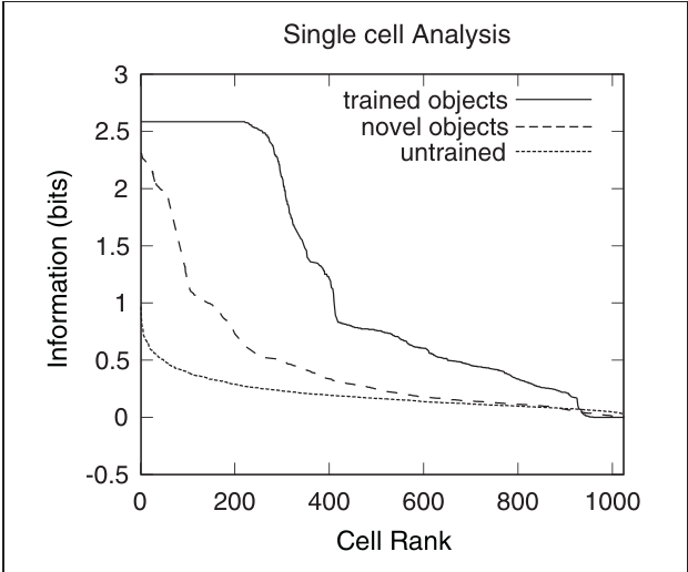
解读：横轴为按不变性排序的第 4 层细胞秩次，纵轴为单细胞信息量（bits）。实线（训练网络测原六物体）有一大批细胞达到最大值 2.58 bits（= log2 6）；虚线（测新物体）信息明显更低、没有细胞达到最大值；点线（随机未训练网络）是基线。这张图把个例细胞的结果推广到群体水平，量化了"排他性不变细胞确实大量存在"。

图 19 · 多细胞信息分析

原文图注：FIGURE 19 | Multiple cell information results obtained when VisNet was tested with the occluded object and five occluding objects rotating through 360° in 1° steps. Multiple cell information analysis results are also plotted for six novel objects that the network was not previously trained on. These novel objects were rotating in the same positions as the six objects on which the network was originally trained. Results are presented after training the network (unbroken line), after testing the trained network with the novel set of objects (dashed line) and with a random untrained network (dotted line). After the network was trained, over 2.5 bits of information was reached, which was substantially higher than 1.10 bits reached by the untrained network or 1.7 bits reached by the trained network that was tested on the novel set of objects. This confirmed that, after training the network, there were cells that form object specific representations to each one of the six objects and do not respond to the object locations.

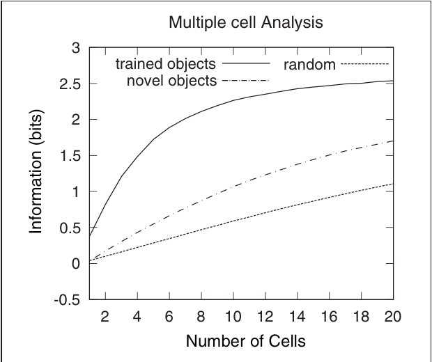
解读：横轴为纳入解码的细胞数（2–20 个），纵轴为多细胞信息量。训练网络测原物体（实线）超过 2.5 bits（接近理论上限），明显高于未训练网络的 1.10 bits 与测新物体的 1.7 bits。它回答了单细胞分析覆盖不到的问题：六个物体确实各自由不同的细胞子集表征，没有任何两个物体共用编码——从分布式读出的角度完成了最后一道验证。

讨论

作者把结果放回"自然视觉中的无监督学习"这一大问题里：与依赖分割、模板匹配或关键特征的人工视觉系统不同，这个生物合理的前馈层级模型靠统计独立性加 CT 学习，就在"被遮挡物从未完整出现"的条件下同时完成了物体分离与部分视图绑定，残余的新物体响应也可以用竞争网络按输入相似度泛化的固有性质解释。结论的可靠性来自三重检验的交叉印证：不变响应、同位置新物体测试失败、碎片视图测试成功，共同排除"位置编码"与"关键标记"两种平凡解。

局限与展望作者写得很具体。其一，计算开销导致只有 Jaimoid 被遮挡，理论上预测更多物体互遮挡时同样可行但未验证；遮挡比例的上限（物体要露出多少才能学成）也待测定。其二，刺激是简单几何形状，这是为了保留回答"how"所需的控制度；作者相信换成复杂物体不会改变结果的定性面貌，但需确认。其三，只测了 CT 学习，trace 学习（时间连续性路线）能否得到同样结果尚未测试。其四，也是最实质的局限：CT 学习依赖物体间因独立运动产生的统计解耦——如果物体完全静止（比如照片里的人脸互相遮挡），当前模型无法把它们分开；作者提到其实验室已用脉冲神经网络动力学（依赖发放时序的突触可塑性，Bi & Poo 1998）解决了这个更难的静态情形，但那属于另一项工作。此外，物体跨视网膜平移（视线扫视场景时的自然情形）被认为原则上可用相同原理解决，文中只是假设、未做模拟。

一句话总结

在我看来，这篇论文的巧妙之处在于把"遮挡"从识别阶段的困难变成了学习阶段的考题：物体永远不完整地出现，反而成了检验不变表征是"记碎片"还是"记整体"的天然试金石——细胞 (4,17) 对五组碎片的响应与对整脸完全一致这一点，比任何信息量指标都更有说服力。CT 学习只靠 Hebb 规则就能做到这一点让我印象深刻，但读者要记住它的适用边界：物体之间得有独立运动来提供统计解耦，静止场景里的遮挡学习是另一套（脉冲时序依赖）机制的事——这是我的理解。

审校与证据追溯 (Verification & Evidence)

图表审计结果

Fig1: 提取质量 good，对齐度 full，识别面板 []
Fig10: 提取质量 good，对齐度 full，识别面板 [A]
Fig11: 提取质量 good，对齐度 full，识别面板 []
Fig12: 提取质量 good，对齐度 full，识别面板 []
Fig13: 提取质量 good，对齐度 full，识别面板 []
Fig14: 提取质量 good，对齐度 full，识别面板 [A]
Fig15: 提取质量 good，对齐度 full，识别面板 []
Fig16: 提取质量 good，对齐度 full，识别面板 []
Fig17: 提取质量 good，对齐度 full，识别面板 []
Fig18: 提取质量 good，对齐度 full，识别面板 []
Fig19: 提取质量 good，对齐度 full，识别面板 []
Fig2: 提取质量 good，对齐度 full，识别面板 []
Fig3: 提取质量 good，对齐度 full，识别面板 []
Fig4: 提取质量 good，对齐度 full，识别面板 []
Fig5: 提取质量 good，对齐度 full，识别面板 []
Fig6: 提取质量 good，对齐度 full，识别面板 []
Fig7: 提取质量 good，对齐度 full，识别面板 []
Fig8: 提取质量 good，对齐度 full，识别面板 []
Fig9: 提取质量 good，对齐度 full，识别面板 []