IT Literature Intelligence 终审版本 (VERIFIED) 论文编号:
194| 原始基线:V0_ZCODE_BASELINE| 语义审核:needs_revision| 图表审核:pass
Invariant visual object and face recognition: neural and computational bases, and a model, VisNet
Rolls · Frontiers in Computational Neuroscience · 2012 · Zotero itemID=1811
一句话定位:这是 Rolls 对自己三十余年工作的集大成式综述,主题是"视觉系统如何在大小、位置、视角、光照不断变化时仍认得同一个物体或面孔"。文章先归纳猕猴下颞叶皮层(inferior temporal cortex, IT)神经元不变表征(invariant representation)的神经生理证据,再以特征层级(feature hierarchy)模型 VisNet 给出计算实现:靠层间会聚的竞争网络加上带短时记忆痕迹的 Hebb 学习规则(trace learning rule),网络就能从自然观看的时空统计中自组织出不变表征。对做视觉计算模型的人,这是一份把"不变性学习、特征绑定、自然场景、注意、海马空间表征"串成一套原理的总纲式文献。
研究背景
物体识别的根本难题在于:同一物体在视网膜上产生的图像随位置、大小、视角、光照而千变万化,而识别必须把这些图像映射到同一组神经元上去。这个问题之所以要紧,是因为一旦视觉系统给出不变表征,下游系统只需一次学习就能把"这个物体"与奖惩、位置、熟悉度等关联起来,并自然泛化到该物体的其他变换形态。当时的神经生理事实是:猕猴 IT 区存在对平移、大小、视角相对独立的响应,且这些区还包含视角依赖与视角不变的混合表征、对特征空间构型敏感的神经元,以及稀疏分布式编码。但"这些不变表征是怎么学出来的"一直没有令人满意的理论——单层点积网络天生只会按相关性泛化、不会平移不变;结构描述(如 Marr 的广义锥、Biederman 的 geon)依赖语法绑定与分割,难以生物实现;模板对齐则需要脑无法胜任的高精度矩阵变换。
另一方面,机器学习侧的各类方案(特征空间列表、map-seeking circuit、可重构输入的网络等)要么忽略特征的空间排列,要么缺乏生物合理性。特征层级方法(从 Neocognitron 到后来的 HMAX)虽然方向与灵长类腹侧通路一致,但既有版本要么靠手工硬编码复杂细胞的不变性、要么靠非局部复制机制,没有说明不变性如何通过一个局部、自组织的学习规则自然涌现。这构成了本文要补上的核心缺口。
研究思路
作者的策略是"神经生理事实约束计算理论,模拟检验理论"。他先系统整理 IT 区数据,提炼出四条工作假设:视觉皮层是 V1→V2→V4→TEO→TE 的层级会聚结构,感受野每级约扩大 2.5 倍;每层是局部自组织竞争网络(相互抑制范围内竞争);用带时间痕迹的修正 Hebb 规则学习;每次只学低阶(2–4 个)特征组合以避免组合爆炸。核心洞察是:真实世界中物体在时空上连续——几秒内看到的往往还是同一个物体的不同变换形态——因此让突触保留约 0.5 秒的活动痕迹,就能把"同一个物体刚刚的样子"与"现在的样子"绑定到同一神经元上,而不把不同物体错误地关联起来。
整篇文章随这条主线逐层展开:先用 T/L/+ 与人脸刺激验证平移不变性和视角不变性的学习;再比较不同形式的 trace 规则及其与误差校正、时间差分学习的数学关系;然后逐一攻克特征绑定、杂乱背景、部分遮挡、3D 深度旋转变换、自然场景中的注意与多物体表征、背侧通路的全局运动不变性;最后把同一原理延伸到海马空间场景表征,并与 HMAX 在标准数据库上做容量对比。图 1 的会聚架构图就是全部讨论的骨架。
方法
改为“本文综述多项既往猕猴IT/STS记录研究,包括注视任务和自然场景搜索任务;各研究样本量与具体设计不同,本文无统一样本量”。,比较有效刺激在不同位置、大小、视角、背景下的放电率;用信息论方法(单细胞信息、总体信息、发放率与同步携带信息的分解)量化表征。模拟部分使用 VisNet:四层各 32×32 神经元(放大版 VisNetL 为 128×128),输入层是模拟 V1 简单细胞的 Gabor/DOG 滤波器组(8 个空间频率 0.0039–0.5 周期/像素逐倍频程、4 个取向步长 45°、正负相位分开),第 1 层每个细胞按高斯分布从前一层局部区域随机采样连接(VisNetL 中第 1 层 272 条连接、各层会聚半径 24/24/36/48,层间边界用环面绕接消除边缘效应);层内用侧抑制滤波器(参数 δ 控制抑制量、σ 控制范围)加 sigmoid 激活函数实现竞争,阈值按每层百分位设定以控制发放稀疏度。
学习规则是全文的重心。基线 trace 规则为 δwj = α·ȳτ·xj,其中痕迹 ȳτ = (1−η)yτ + η·ȳτ−1 以指数衰减;性能用 Fisher 判别因子(对刺激的区分度相对对位置的区分度之比,>1 表示不变)与信息论量度(单细胞信息、多细胞信息,后者经 Bayes 解码计算,上限为 log2 刺激数)评估。后续版本包括无当前项痕迹的修改 trace 规则(δwj = α·ȳτ−1·xj)、五种以邻近时刻活动为目标值的误差校正规则、以及把目标/输入项改为加权和的 TD(λ) 型规则,各自在"7 张脸 × 9 个位置"等问题上做参数优化后比较。
主要结果
- IT 区不变表征的神经生理画像:许多神经元对刺激的响应相对独立于视网膜位置与大小(平均半最大响应跨度约 12 倍,即 3.5 倍频程;而 V1 约 1.5 倍频程),部分神经元在低通/高通滤波至仅含 8 周期/脸时仍响应;同一皮层区内混有视角依赖、部分视角不变与完全视角不变的神经元(如 18 个里 16 个并非完全视角不变);许多神经元只对多个特征按正确空间构型组合出现时响应(图 5、图 6)。表征是稀疏分布式的,信息随神经元数目近似线性增长,且 94–99% 的信息在发放率中、刺激依赖同步携带的信息不足 5%。
- VisNet 学会不变表征且不变性逐层递增:T/L/+ 实验中第 1 层神经元判别因子仅 1.04(组合特征、位置特异),第 4 层达 4.07 与 3.62(图 12–14);7 张脸 × 9 个位置训练后判别因子沿四层递增(图 15);trace 规则是决定因素——纯 Hebb 学习的结果甚至比随机权重还差,因为它学出的是位置分析器而非物体分析器(图 16);3 张脸 × 7 个视角的中心呈现实验中第 4 层判别因子达 11.12、12.40(图 17)。
- 学习规则的谱系与最优形式:无当前项痕迹的规则 (17) 显著优于标准 trace 规则 (14)(图 18);五种误差校正规则全部优于两者,其中含痕迹目标、不含当前发放的规则 (21) 最好;TD(λ) 型推广中 TD(1) 型规则 (38)(λ=1,β=1.8)给出最好的单细胞信息,把不变性学习与时间差分学习正式联系起来。
- 特征绑定、杂乱背景与遮挡:补充“除RTL和TLBR外,其余刺激在全部测试位置达到完全平移不变”。(如 TL 不会被 T 或 TLB 误触发,图 19–21,单细胞信息达 log2 6 = 2.6 bits 上限),并泛化到训练时未出现的位置;已学物体在杂乱背景下测试几乎无损,但在杂乱背景中学习新物体需要某种分割(可用先前暴露、中央凹优势或注意来补救,图 22);改为“单细胞信息仅小幅下降,但遮挡上半脸时多细胞信息停留在次优水平;露出上半脸的条件表现更好”。,且露出上半脸时更好,与心理学一致(图 23);3D 深度旋转的表面特征透视变换可被 trace 学习掌握,三元组只在 4 个视角训练即可在 5 个视角不变识别(图 24、25)。
- 机制解释、扩展与容量:自然场景中 IT 感受野从单刺激空白背景的 77.6° 缩到 22.0°(作为动作目标时 19.2°),而空白背景中物体注意可把感受野从 17.2° 扩到 47.0°——吸引子网络模型用中央凹放大因子加权解释了这一切(图 30–33);同一原理推广到背侧通路产生位置与尺寸不变的全局运动表征(图 38),加第五层可自组织出海马 spatial view/place 细胞(图 39);放大版 VisNetL 在 ALOI 数据库上优于规模相当化的 HMAX_min(χ²=110.58, df=1, p=10⁻³),训练视角间隔 45° 即可泛化到离最近训练视角 22.5° 的测试视角,而 Caltech-256 因类内样本不连续而不适合训练不变表征(图 41–44)。
图注解读
图 1 · 视觉系统的会聚架构
原文图注:FIGURE 1 | Convergence in the visual system. Right – as it occurs in the brain. V1, visual cortex area V1; TEO, posterior inferior temporal cortex; TE, inferior temporal cortex (IT). Left – as implemented in VisNet. Convergence through the network is designed to provide fourth layer neurons with information from across the entire input retina.
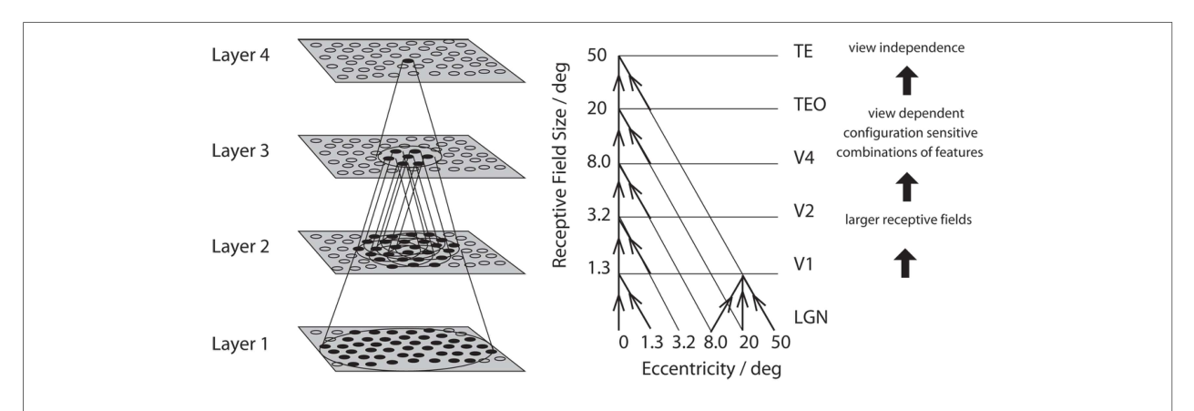
解读:左右对照图:右边是脑中 V1→V2→V4→TEO→TE 的逐级会聚,左边是 VisNet 四层的对应实现。要点是感受野逐级扩大(V1 约 1°、V4 约 8°、TEO 约 20°、IT 约 50°)且会聚区连续重叠,使顶层神经元能接收来自整个输入"视网膜"的信息——这是平移不变性的架构基础,也是全文所有模拟的骨架。
图 2 · 猕猴颞叶皮层分区图
原文图注:FIGURE 2 | Lateral view of the macaque brain (left hemisphere) showing the different architectonic areas (e.g., TEm, TEa) in and bordering the anterior part of the superior temporal sulcus (STS) of the macaque (see text). The STS has been drawn opened to reveal the cortical areas inside it, and is circumscribed by a thick line.
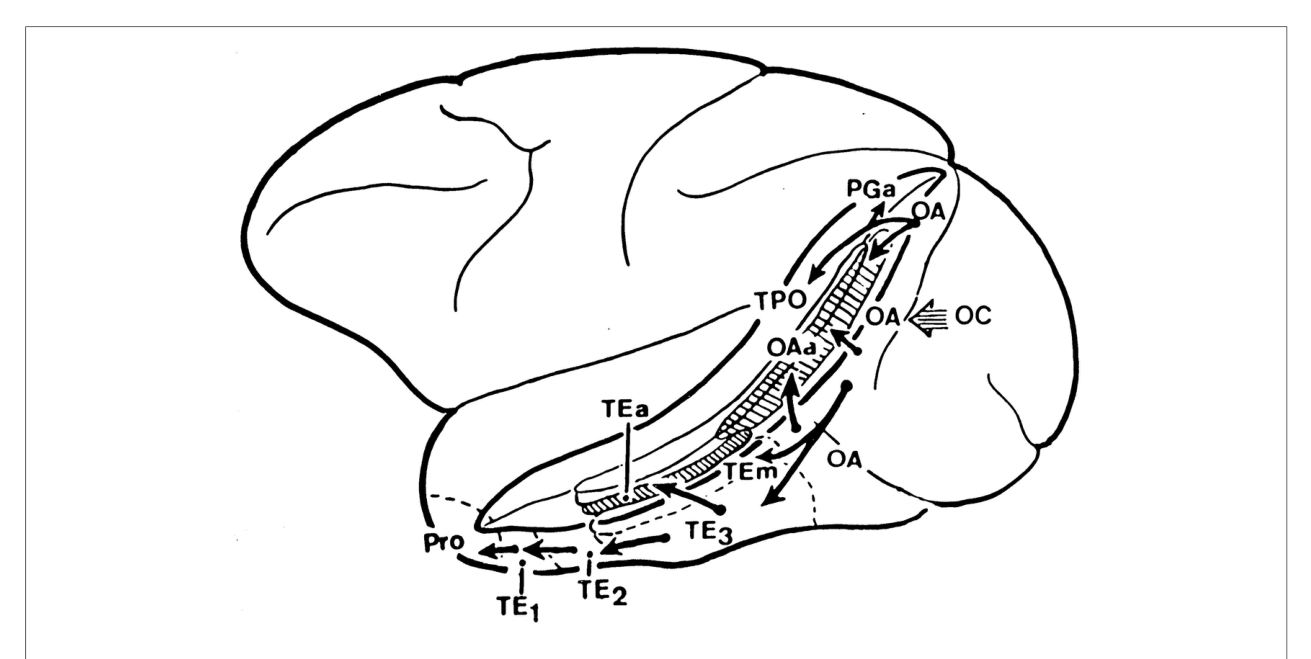
解读:猕猴左半球侧面视图,上颞沟(STS)被剖开以显示沟内分区(TEm、TEa 等)。它为第 2 节的神经生理证据提供解剖坐标:面孔身份、表情/运动、物体分别位于不同的亚区,文中记录的有效刺激神经元主要在蝶骨参照点后 7–3 mm、距耳间平面 11–15 mm 之前的区域。
图 3 · 自然场景中的多物体混淆问题
原文图注:FIGURE 3 | Objects shown in a natural scene, in which the task was to search for and touch one of the stimuli. The objects in the task as run were smaller. The diagram shows that if the receptive fields of inferior temporal cortex neurons are large in natural scenes with multiple objects (in this scene, bananas, and a face), then any receiving neuron in structures such as the orbitofrontal cortex and amygdala would receive information from many stimuli in the field of view, and would not be able to provide evidence about each of the stimuli separately.
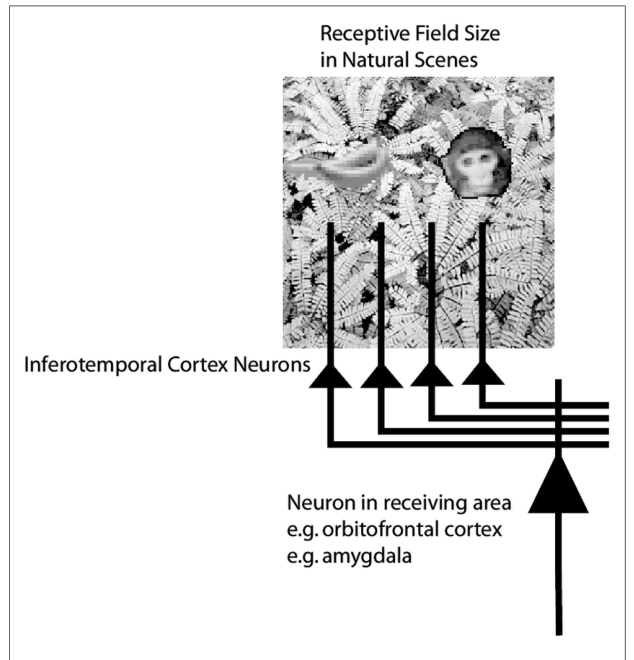
解读:示意图给出一个关键问题的提出:场景里有香蕉和一张脸,若 IT 神经元感受野很大,那么眶额皮层、杏仁核等下游结构收到的将是视野内多个刺激的混合信号,无法分别对每个刺激做出奖惩关联。这张图引出"自然场景中平移不变性应当受限"的核心主张,后面图 4、31、33 都在回答它。
图 4 · 注视偏离时自然场景响应衰减
原文图注:FIGURE 4 | Firing of a temporal cortex cell to an effective stimulus presented either in a blank background or in a natural scene, as a function of the angle in degrees at which the monkey was fixating away from the effective stimulus. The task was to search for and touch the stimulus. (After Rolls et al., 2003.)
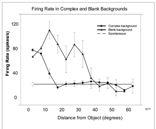
解读:横轴是注视点偏离有效刺激的角度,纵轴是该颞叶皮层细胞的放电,曲线分空白背景与自然场景两种条件。自然场景中响应随偏离角度迅速衰减、空白背景中衰减缓慢,直接支撑"自然场景中 IT 感受野缩小到约物体大小"的结论,也解释了视觉系统为何以注视点为界面向动作系统输出。
图 5 · 大小不变性示例
原文图注:FIGURE 5 | Typical response of an inferior temporal cortex face-selective neuron to faces of different sizes. The size subtended at the retina in degrees is shown. (From Rolls and Baylis, 1986.)
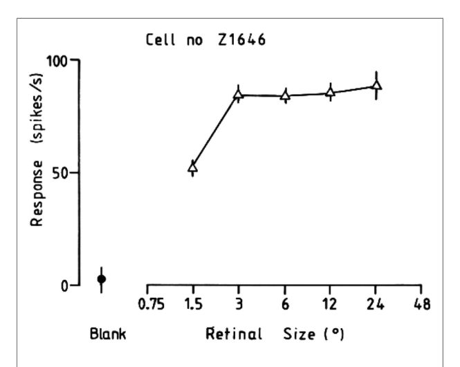
解读:单个 IT 面孔选择神经元对以不同视网膜视角大小呈现的脸的响应曲线,峰值区域覆盖很宽。群体平均的半最大响应跨度约为 12 倍(3.5 倍频程),远超 V1 神经元的约 1.5 倍频程——单层点积网络给不出这种性质(见下一条图),这是层级加工必要性的直接证据。
图 6 · 特征组合与正确空间构型的敏感性
原文图注:FIGURE 6 | Responses of four temporal cortex neurons to whole faces and to parts of faces. The mean firing rate ± sem are shown. The responses are shown as changes from the spontaneous firing rate of each neuron. Some neurons respond to one or several parts of faces presented alone. Other neurons (of which the top one is an example) respond only to the combination of the parts (and only if they are in the correct spatial configuration with respect to each other as shown by Rolls et al., 1994). The control stimuli were non-face objects. (After Perrett et al., 1982.)
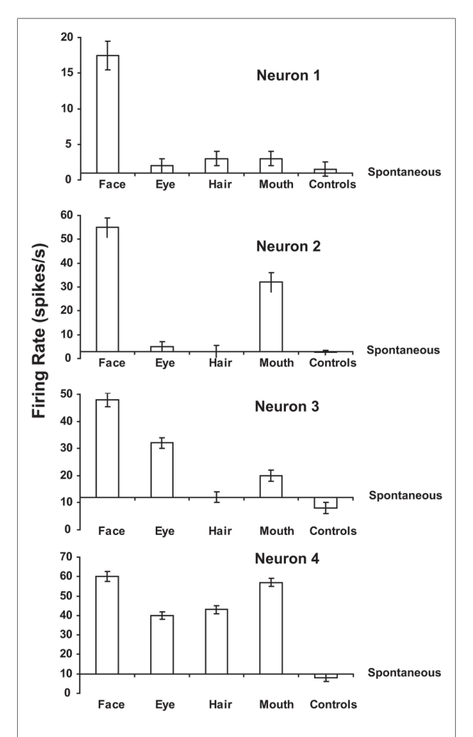
解读:四个神经元对整脸、脸部件(单独呈现的眼、发、口等)与非脸对照物的响应(相对自发放电的变化,均值±SEM)。最上面的神经元只对"全部部件按正确空间构型组合"响应,其余对个别部件也响应。这张图把"特征组合神经元"的概念落到实处,是 VisNet 低阶组合假设的神经生理依据。
图 7 · 单层点积网络没有平移不变性
原文图注:FIGURE 7 | A neuron that computes a dot product of the input pattern with its synaptic weight vector generalizes well to other patterns based on their similarity measured in terms of dot product or correlation, but shows no translation (or size, etc.) invariance.
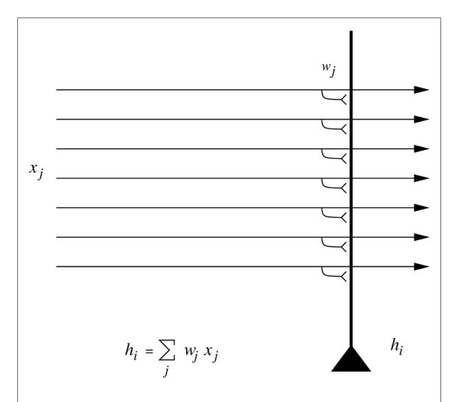
解读:一个按激活 hi = Σj xj·wij 工作的神经元对与已学模式相关性高的输入泛化良好,但把输入平移一位,点积即跌到低值、神经元不再响应。这张"反例图"用来立论:不变性不是网络的默认属性,需要专门机制——全文由此展开。
图 8 · Marr 与 Nishihara 的结构描述方案
原文图注:FIGURE 8 | A 3D structural description of an object-based on generalized cone parts. Each box corresponds to a 3D model, with its model axis on the left side of the box and the arrangement of its component axes on the right. In addition, some component axes have 3D models associated with them, as indicated by the way the boxes overlap. (After Marr and Nishihara, 1978.)
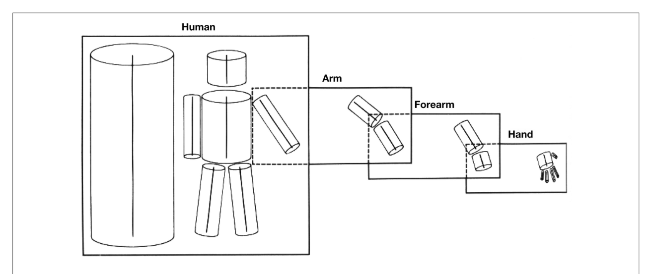
解读:基于广义锥部件的 3D 结构描述层级:每个方框对应一个 3D 模型,左侧是模型轴、右侧是组件轴的排布,部分框之间重叠表示组件轴也带 3D 模型。它代表"先分解部件、再建结构描述、后与存储模板匹配"的路线;正文列举了分解困难、语法绑定难以生物实现等五大难题,结论是脑不太可能走这条路。
图 9 · 特征层级方法的示意图
原文图注:FIGURE 9 | The feature hierarchy approach to object recognition. The inputs may be neurons tuned to oriented straight line segments. In early intermediate-layers neurons respond to a combination of these inputs in the correct spatial position with respect to each other. In further intermediate layers, of which there may be several, neurons respond with some invariance to the feature combinations represented early, and form higher order feature combinations. Finally, in the top layer, neurons respond to combinations of what is represented in the preceding intermediate layer, and thus provide evidence about objects in a position (and scale and even view) invariant way. Convergence through the network is designed to provide top layer neurons with information from across the entire input retina, as part of the solution to translation invariance, and other types of invariance are treated similarly.
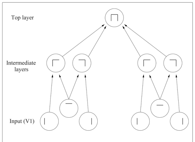
解读:从取向线段检测器出发,早中间层响应正确相对位置的特征组合,后续中间层带一定不变性地组合出更高阶特征,顶层以位置(及尺度、视角)不变的方式给出"是哪个物体"的证据。这是 VisNet 所代表路线的总示意,与图 1 呼应。
图 10 · 侧抑制对比增强滤波器
原文图注:FIGURE 10 | Contrast-enhancing filter, which has the effect of local lateral inhibition. The parameters δ and σ are variables used in equation (5) to modify the amount and extent of inhibition, respectively.
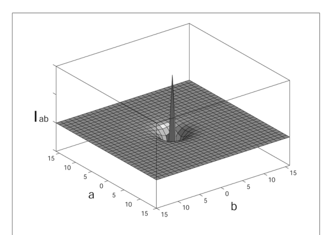
解读:实现层内竞争的空间滤波器:中心兴奋、周边抑制,δ 控制抑制强度、σ 控制抑制范围。它让"接收相似输入的过多神经元"彼此竞争,保证不同神经元编码不同输入、降低冗余——VisNet 每层的第一步运算。
图 11 · 滤波器采样范式
原文图注:FIGURE 11 | The filter sampling paradigm. Here each square represents the retinal image presented to the network after being filtered by a Gabor filter of the appropriate orientation sign and frequency. The circles represent the consistent retinotopic coordinates used to provide input to a layer 1 cell. The filters double in spatial-frequency toward the reader. Left to right the orientation tuning increases from 0° in steps of 45°, with segregated pairs of positive (P) and negative (N) filter responses.
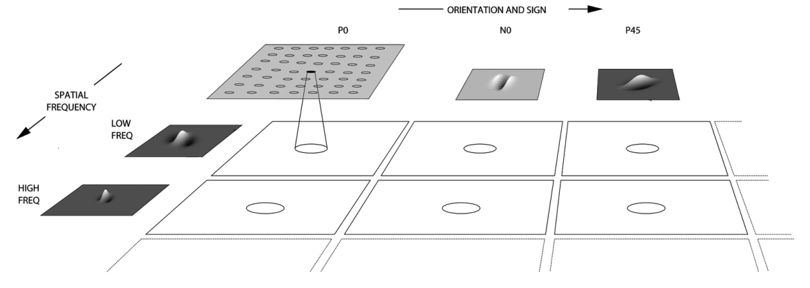
解读:每个方格是经某 Gabor 滤波器(按取向列、按空间频率行排列,P/N 正负输出分开)过滤后的视网膜图像,圆圈标出第 1 层一个细胞的一致视网膜拓扑采样坐标。空间频率朝读者方向逐倍频程翻倍、取向从 0° 以 45° 步进。读这张图就明白 VisNet 的"V1 输入"长什么样。
图 12 · 第 1 层神经元仍是位置特异的组合检测器
原文图注:FIGURE 12 | The left graph shows the response of a layer 1 neuron to the three training stimuli for the nine training locations. Alongside this are the results of summating all the filter inputs to the neuron. The discrimination factor for this cell was 1.04.
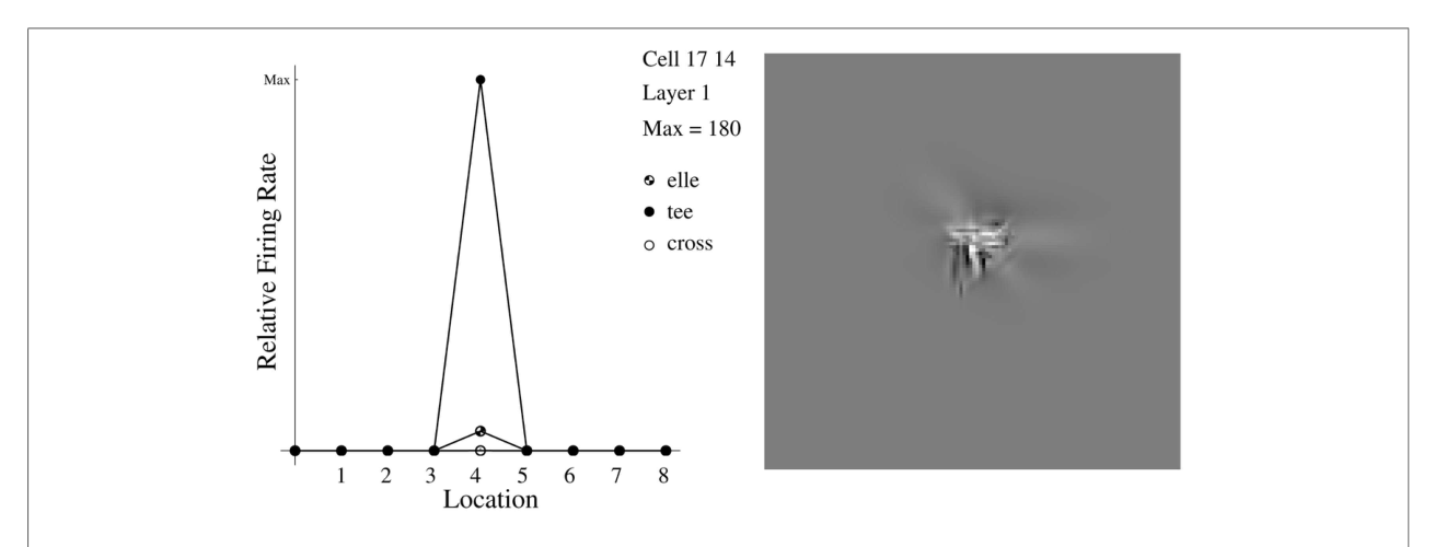
解读:左侧为一个第 1 层神经元对 T/L/+ 三刺激在九个训练位置的响应,右侧是所有滤波器输入的加权和。判别因子只有 1.04——略高于 1,说明这一层的神经元学到了"特征组合"(能区分 T 与 L/+),但几乎没有平移不变性。这正符合设计意图:组合与精确空间信息要在不变性出现之前先形成。
图 13 · 训练后第 1 层细胞的连接模式
原文图注:FIGURE 13 | The connections to a single cell in layer 1 of VisNet from the filters after training in the T, L, and + stimulus set, represented by plotting the receptive fields of every input layer cell connected to the particular layer 1 cell. Separate input layer cells have activity that represents a positive (P) or negative (N) output from the bank of filters which have different orientations in degrees (the columns) and different spatial frequencies (the rows). Here the overall receptive field of the layer 1 cell is centered just below the center-point of the retina. The connection scheme allows for relatively fewer connections to lower frequency cells than to high-frequency cells in order to cover a similar region of the input at each frequency. The blank squares indicate that no connection exists between the layer 1 cell chosen and the filters of that particular orientation, sign, and spatial-frequency.
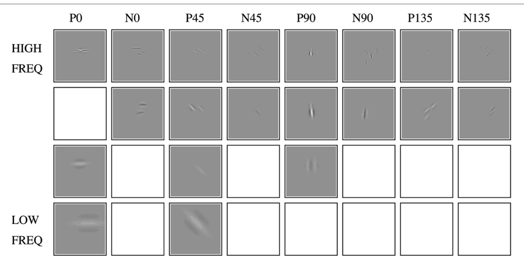
解读:把与该第 1 层细胞相连的每个输入单元的感受野都画出来,列按滤波器取向、行按空间频率排布。训练后许多低频滤波器连接被压到零、只保留相关取向,空白方格表示连接不存在。它是图 12 结论的机制展示:学习从随机布线收敛为稀疏而有序的特征组合连接。
图 14 · 第 4 层出现平移不变的刺激识别
原文图注:FIGURE 14 | Response profiles for two fourth layer neurons – discrimination factors 4.07 and 3.62 – in the L, T, and + experiment.
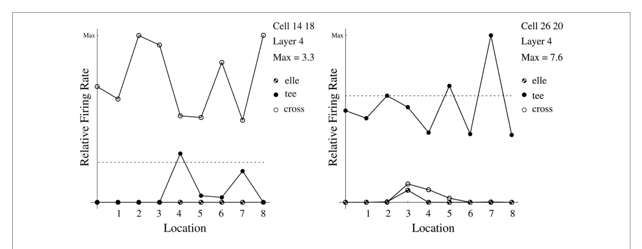
解读:两个第 4 层神经元的响应轮廓(判别因子 4.07 与 3.62):对同一个刺激在全部九个位置响应都高、对其他刺激在所有位置都低。与图 12 的 1.04 对比,平移不变、刺激特异的表征确实在顶层出现了。
图 15 · 不变性沿层级递增
原文图注:FIGURE 15 | Variation in network performance for the top 30 most highly discriminating cells through the four layers of the network, averaged over five runs of the network. The net was trained on 7 faces each in 9 locations.
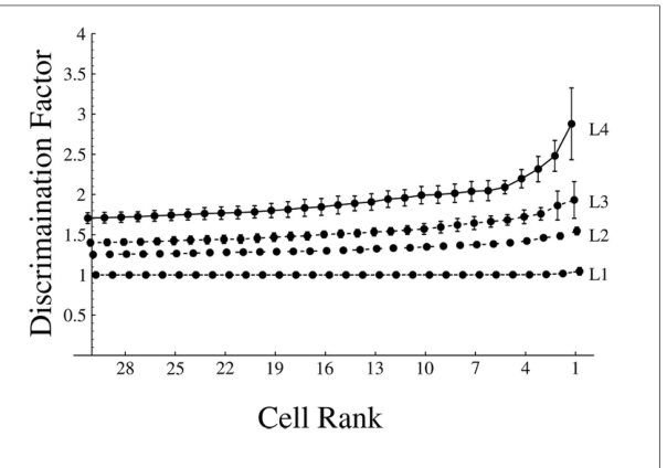
解读:7 张脸各 9 个位置训练,取每层判别能力最高的 30 个细胞的判别因子(5 次运行平均)画柱状对比。第 1 到第 4 层不变性逐层上升,与"每层学一点不变性、逐层累积"的架构假设一致。
图 16 · trace 规则是决定性因素
原文图注:FIGURE 16 | Variation in network performance for the top 30 most highly discriminating cells in the fourth layer for the three training regimes, averaged over five runs of the network. The net was trained on 7 faces each in 9 locations.
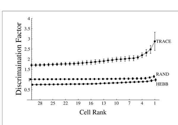
解读:第 4 层 top 30 细胞在三种训练制度下的对比:trace 规则、未训练(随机权重)、η=0 的纯 Hebb 规则。结果反直觉但信息量大——纯 Hebb 甚至比随机还差:因为同一图像在同一位置的重复出现使 Hebb 网络按"在哪里"而非"是什么"分类。trace 规则由此被确立为不变性学习的核心。
图 17 · 视角不变表征的响应轮廓
原文图注:FIGURE 17 | Response profiles for cells in the last two layers of the network – discrimination factors 11.12 and 12.40 – in the experiment with seven different views of each of three faces.
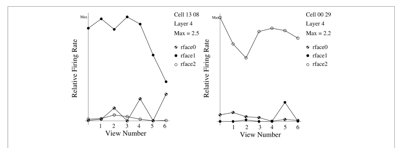
解读:3 张脸各 7 个视角(共 21 个视角,全部在中心重叠呈现,比平移问题更难)训练后的最后两层神经元响应轮廓,判别因子高达 11.12 与 12.40。说明 trace 学习同样能解决"非同构变换"的视角不变性问题。
图 18 · 各种学习规则的数值比较
原文图注:FIGURE 18 | Numerical results with the standard trace rule (14), the modified trace-learning rule (17), the Hebb rule (16), and random weights, trained on 7 faces in 9 locations: single cell information measure (left), multiple cell information measure (right). (After Rolls and Stringer, 2001a.)
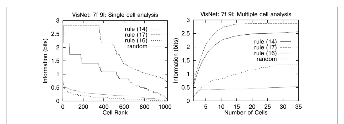
解读:7 脸 × 9 位置训练下四种制度(标准 trace (14)、修改 trace (17)、Hebb (16)、随机权重)的单细胞信息(左)与多细胞信息(右)排名曲线。修改 trace 规则 (17)——痕迹只取前一时刻、不含当前发放——明显优于标准 trace,为后续误差校正与时序差分规则的推广提供了出发点。
图 19 · 子集/超集刺激全集
原文图注:FIGURE 19 | Merged feature objects. All members of the full object set are shown, using a dotted line to represent the central 32 × 32 square on which the individual features are positioned, with the features themselves shown as dark line segments. Nomenclature is by acronym of the features present, where T, top; B, bottom; L, left; and R, right. (After Elliffe et al., 2002.)
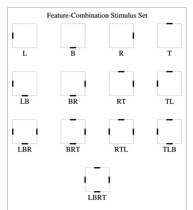
解读:实验刺激全集:四条 8×1 条形(上 T、下 B、左 L、右 R)在中央 32×32 方区内自由组合出的所有物体,按包含特征数分组(单个、两个、三个、四个特征),以特征缩写命名(如 LBR、TL)。这套"共同特征字母表"专门用来检验网络能否区分彼此为子集/超集的刺激——不是靠某个独特特征投机取巧。
图 20 · 三特征三位置的组合命名法
原文图注:FIGURE 20 | Feature combinations for experiments of Section 5.4.5: there are 3 features denoted by 1, 2, and 3 (including a blank space 0) that can be placed in any of 3 positions A, B, and C. Individual stimuli are denoted by three consecutive numbers which refer to the individual features present in positions A, B, and C, respectively. In the experiments in Section 5.4.5, layers 1 and 2 were trained on stimuli consisting of pairs of the features, and layers 3 and 4 were trained on stimuli consisting of triples. Then the network was tested to show whether layer 4 neurons would distinguish between triples, even though the first two layers had only been trained on pairs. In addition, the network was tested to show whether individual cells in layer 4 could distinguish between triples even in locations where the triples were not presented during training. (After Elliffe et al., 2002.)
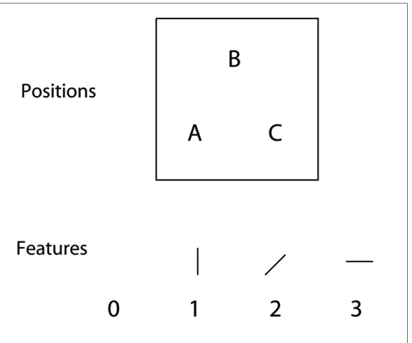
解读:特征 1(垂直)、2(对角)、3(水平)可放在 A/B/C 三个位置(0 为空位),刺激用三位数命名(如 102、123),共 18 个对与 6 个三元组。实验设计:第 1、2 层只训"对"、第 3、4 层训"三元组",然后检验第 4 层能否区分三元组(包括在未训练位置上)。这是特征绑定问题最严格的操作化。
图 21 · 绑定实验的信息量结果
原文图注:FIGURE 21 | Numerical results for experiments 1–4 as described in Table 5, with the trace-learning rule (17). On the left are single cell information measures, and on the right are multiple cell information measures. (After Elliffe et al., 2002.)
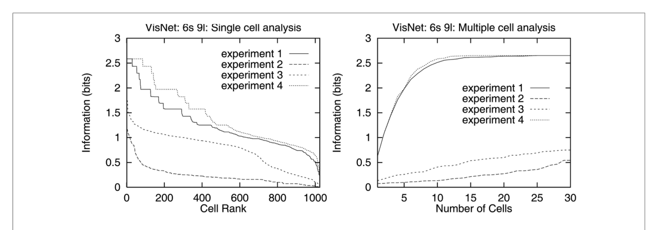
解读:四种训练制度(实验 1:低层训对+高层训三元组;实验 2:全不训;实验 3:仅高层训三元组;实验 4:全部训三元组)下第 4 层的单细胞信息(左)与多细胞信息(右)。实验 1 多个细胞达到 log2 6 = 2.6 bits 的理论上限,优于实验 3、几乎追平实验 4——证明早期层形成的"部分不变的特征对"足以支撑高层对完整空间排列的判别,特征绑定问题在层级网络内得到解决。
图 22 · 两个杂乱背景
原文图注:FIGURE 22 | Cluttered backgrounds used in VisNet simulations: backgrounds 1 and 2 are on the left and right, respectively.
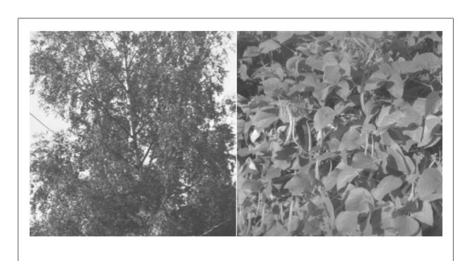
解读:模拟中使用的两个 128×128 像素自然感杂乱背景,面孔刺激在其上 9 个格点位置之一呈现。背景固定不变是该实验的技术设定——它也正是"在杂乱背景中学习新物体效果差"的部分原因(神经元学到了背景而非刺激)。
图 23 · 部分遮挡下的识别
原文图注:FIGURE 23 | Effects of partial occlusion of a stimulus: numerical results for experiment 6 of Stringer and Rolls (2000), with the 7 faces presented on a blank background during both training and testing. Training was performed with the whole face. However, during testing there are two options: either (i) the top half of all the faces are occluded, or (ii) the bottom half of all the faces are occluded. On the left are single cell information measures, and on the right are multiple cell information measures.
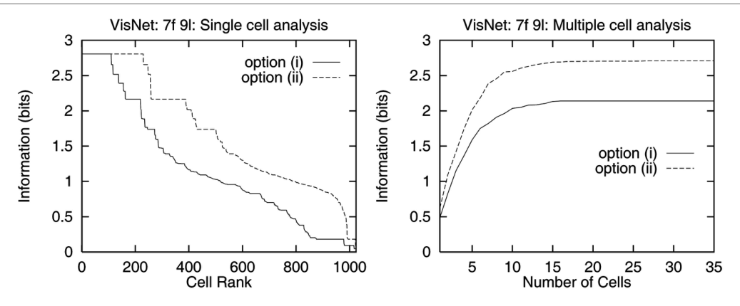
解读:7 张脸整脸训练后,测试时遮挡上半或下半(两个测试条件间无共同特征,排除单特征投机)。左、右分别为单细胞与多细胞信息:与不遮挡相比只有小幅下降,且遮挡下半(露出眼睛、头发等信息更丰富的上半)表现更好,与心理学上"认脸靠上半"的观察一致。分布式表征加联想处理赋予了模型对遮挡的鲁棒性。
图 24 · 3D 透视变换学习刺激
原文图注:FIGURE 24 | Learning 3D perspectival transforms of features. Representations of the 6 visual stimuli with 3 surface features (triples) presented to VisNet during the simulations described in Section 5.6. Each stimulus is a sphere that is uniquely identified by a unique combination of three surface features (a vertical, diagonal, and horizontal arc), which occur in 3 relative positions A, B, and C. Each row shows one of the stimuli rotated through the 5 different rotational views in which the stimulus is presented to VisNet. From left to right the rotational views shown are: (i) –60°, (ii) –30°, (iii) 0° (central position), (iv) +30°, and (v) +60°. (After Stringer and Rolls, 2002.)
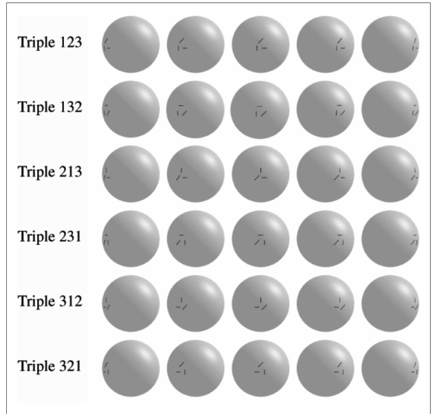
解读:6 个球体刺激,每个由垂直/对角/水平三条弧线在 A/B/C 三个相对位置的独特组合标识,每行展示一个刺激在 −60° 到 +60°(步长 30°)五个深度旋转视角下的投影。表面特征随旋转发生的透视变形正是网络要学习的"第三类变换"——既要在视角间泛化、又不能混淆不同球。
图 25 · 3D 实验的数值结果
原文图注:FIGURE 25 | Learning 3D perspectival transforms of features. Numerical results for experiments 1 and 2: on the left are single cell information measures, and on the right are multiple cell information measures. (After Stringer and Rolls, 2002.)
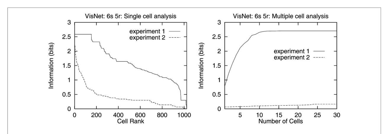
解读:实验 1(低层以"对"训练、高层以三元组训练但只在 4 个视角呈现)对实验 2(不训练基线)的单细胞/多细胞信息对比。三元组只在 4 个视角训练,第 4 层却在全部 5 个视角不变识别,多细胞信息达到 2.6 bits 上限;而用未变形特征训练的对照网络在真实变形特征上失败——说明网络学到的是"表面特征在 3D 旋转中如何变换"的知识本身。
图 26 · VisNet 的 trace 学习方案
原文图注:FIGURE 26 | The learning scheme implemented in VisNet. A trace-learning rule is implemented in the feed-forward inputs to a competitive network.
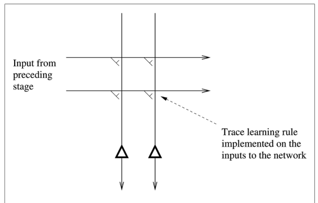
解读:示意图:痕迹学习规则实现于进入竞争网络的前馈突触上,痕迹由后突触神经元自身活动的衰减构成。这是 VisNet 主线模型(与下一条图的循环网络方案相对)的实现位置。
图 27 · 吸引子网络版本的 trace 学习
原文图注:FIGURE 27 | The learning scheme considered by Parga and Rolls (1998) and Elliffe et al. (2000). There are inputs to the network from the preceding stage via unmodifiable synapses, and a trace or pairwise associative learning rule is implemented in the recurrent collateral synapses of an autoassociative memory to associate together the different exemplars (e.g., views) of the same object.
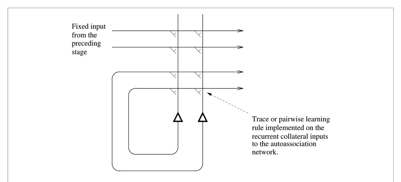
解读:另一套实现位置:前级输入经不可修饰突触进入,trace/成对联合学习改在自联想记忆的循环侧支突触上进行。同一物体的不同视角(例证)在时间上靠近出现时被绑进同一个吸引子——学习后呈现任一视角都会收敛到代表"这个物体"的状态。该方案的优点是可用统计物理方法解析容量。
图 28 · 全视角互连的突触矩阵
原文图注:FIGURE 28 | A schematic illustration of the first type of associations contributing to the synaptic matrix considered by Parga and Rolls (1998). Object 1 (O1) has five views labeled v1 to v5, etc. The matrix is formed by associating the pattern presented in the columns with itself, that is with the same pattern presented as rows.
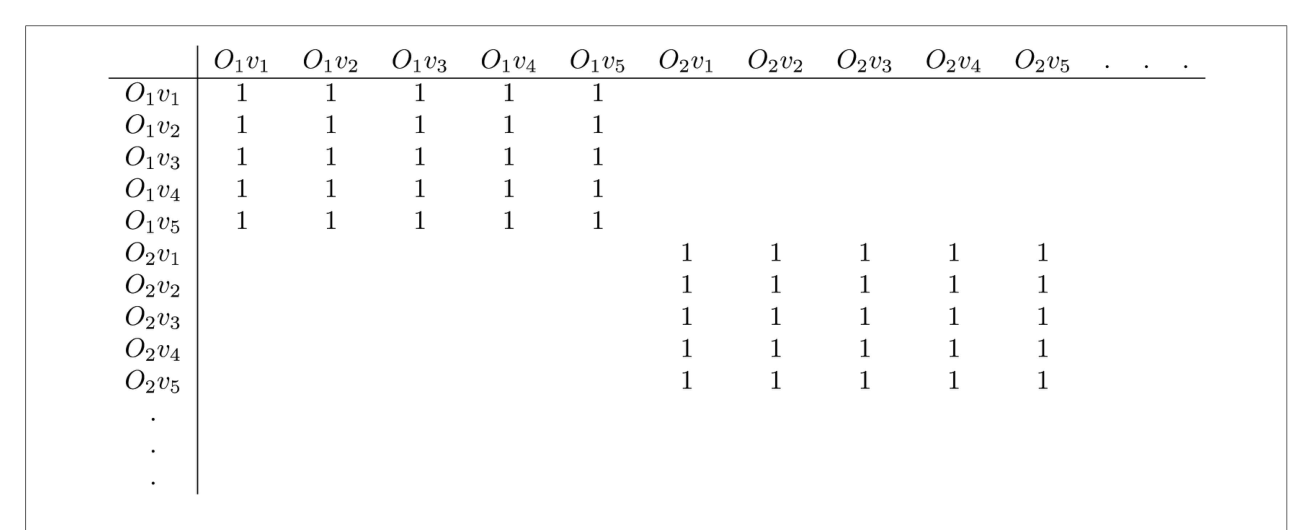
解读:第一类关联矩阵:物体 1 的 5 个视角(v1–v5)两两等强度互连(含自身),形成对角线上的 5×5 值为 1 的方块;物体 2 沿对角再形成另一块。每个物体对应一个由若干视角元素共同构成的 attractor。
图 29 · 成对相邻视角的关联矩阵
原文图注:FIGURE 29 | A schematic illustration of the second and main type of associations contributing to the synaptic matrix considered by Parga and Rolls (1998) and Elliffe et al. (2000). Object 1 (O1) has five views labeled v1 to v5, etc. The association of any one view with itself has strength 1, and of any one with another view of the same object has strength b.
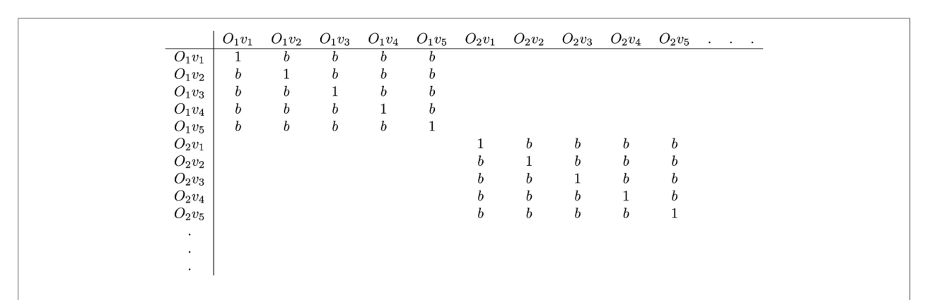
解读:第二类(主要情形)关联矩阵:对角线为 1(自身强化),同一物体的不同视角之间为强度 b。这对应更现实的情形——任意两个视角都可能先后出现而被成对联合,或由指数衰减痕迹产生强度渐弱的跨视角连接。解析结果表明可存物体数随每个神经元的循环连接数线性增长(Po = kC/s,k 约 0.07–0.09;5 个视角时约 0.081N/5)。
图 30 · 视觉搜索任务
原文图注:FIGURE 30 | The visual search task. The monkey had to search for and touch an object (in this case a banana) when shown in a complex natural scene, or when shown on a plain background. In each case a second object is present (a bottle) which the monkey must not touch. The stimuli are shown to scale. The screen subtended 70° × 55° (After Rolls et al., 2003.)
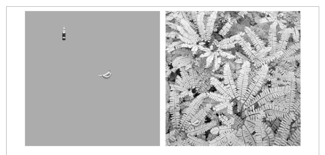
解读:神经生理实验的任务示意:猴子需在复杂自然场景或纯色背景中搜索并触摸目标(香蕉)、避开另一物体(瓶子),刺激按实际比例绘制,屏幕视角 70°×55°。它与图 3 呼应,是"自然场景中物体选择"研究的实验载体。
图 31 · 自然场景与注意下的感受野汇总
原文图注:FIGURE 31 | Summary of the receptive field sizes of inferior temporal cortex neurons to a 5° effective stimulus presented in either a blank background (blank screen) or in a natural scene (complex background). The stimulus that was a target for action in the different experimental conditions is marked by T. When the target stimulus was touched, a reward was obtained. The mean receptive field diameter of the population of neurons analyzed, and the mean firing rate in spikes/s, is shown. The stimuli subtended 5° × 3.5° at the retina, and occurred on each trial in a random position in the 70° × 55° screen. The dashed circle is proportional to the receptive field size. Top row: responses with one visual stimulus in a blank (left) or complex (right) background. Middle row: responses with two stimuli, when the effective stimulus was not the target of the visual search. Bottom row: responses with two stimuli, when the effective stimulus was the target of the visual search. (After Rolls et al., 2003.)
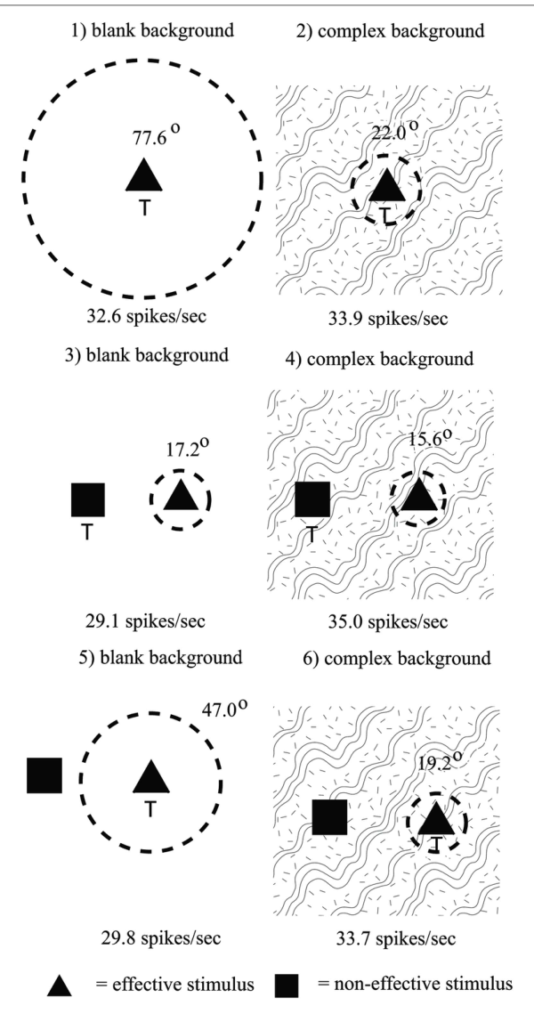
解读:六个条件的感受野直径汇总(虚线圆与感受野大小成比例,标出平均放电率):单个刺激时空白背景 77.6° vs 自然场景 22.0°;两刺激、有效刺激非搜索目标时 15.6°;是目标时 19.2°;而空白背景中注意使感受野从 17.2° 扩到 47.0°。对比之下,自然场景中注意的效应相对很小——"中央凹优先"才是主导原则,这张图是第 5.8 节论证的核心证据。
图 32 · IT 吸引子网络模型架构
原文图注:FIGURE 32 | The architecture of the inferior temporal cortex (IT) model of Trappenberg et al. (2002) operating as an attractor network with inputs from the fovea given preferential weighting by the greater magnification factor of the fovea. The model also has a top-down object-selective bias input. The model was used to analyze how object vision and recognition operate in complex natural scenes.
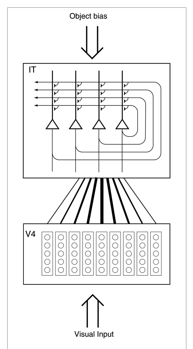
解读:模型架构:V4 以多个 6° 宽的视网膜拓扑模块表示视野,向作为吸引子网络的 IT 投射,来自中央凹模块的输入按皮层放大因子被优先加权,另有自上而下的物体选择偏置输入(强度 k_IT_BIAS)。它把"感受野为什么在自然场景中缩小"归结为:只有靠近中央凹的物体才能赢得吸引子竞争。
图 33 · 模型复现感受野缩小与注意效应
原文图注:FIGURE 33 | Correlations as measured by the normalized dot product between the object vector used to train IT and the state of the IT network after settling into a stable state with a single object in the visual scene (blank background) or with other trained objects at all possible locations in the visual scene (natural background). There is no object bias included in the results shown in graph (A), whereas an object bias is included in the results shown in (B) with k_IT_BIAS = 0.7 in the experiments with a natural background and k_IT_BIAS = 0.1 in the experiments with a blank background. (After Trappenberg et al., 2002.)
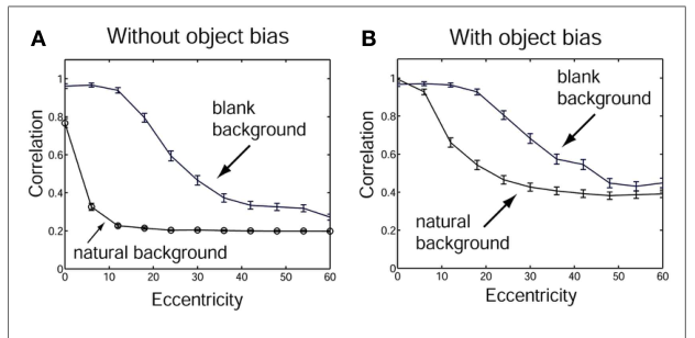
解读:横轴为物体离心位置,纵轴为目标物体向量与网络稳态的归一化点积(识别好坏的度量)。(A) 无注意偏置:空白背景下识别几乎不随位置衰减(感受野大),自然背景下中央凹附近才高(感受野小);(B) 加物体偏置(自然背景 k=0.7、空白背景 k=0.1)后两种背景的感受野都变大,复现了图 31 的注意效应。模型与生理数据在定性上全面吻合。
图 34 · 含注意的皮层级架构
原文图注:FIGURE 34 | Cortical architecture for hierarchical and attention-based visual perception after Deco and Rolls (2004). The system is essentially composed of five modules structured such that they resemble the two known main visual paths of the mammalian visual cortex. Information from the retino-geniculo-striate pathway enters the visual cortex through area V1 in the occipital lobe and proceeds into two processing streams. The occipital-temporal stream leads ventrally through V2–V4 and IT (inferior temporal visual cortex), and is mainly concerned with object recognition. The occipito-parietal stream leads dorsally into PP (posterior parietal complex), and is responsible for maintaining a spatial map of an object's location. The solid lines with arrows between levels show the forward connections, and the dashed lines the top-down backprojections. Short-term memory systems in the prefrontal cortex (PF46) apply top-down attentional bias to the object or spatial processing streams. (After Deco and Rolls, 2004.)
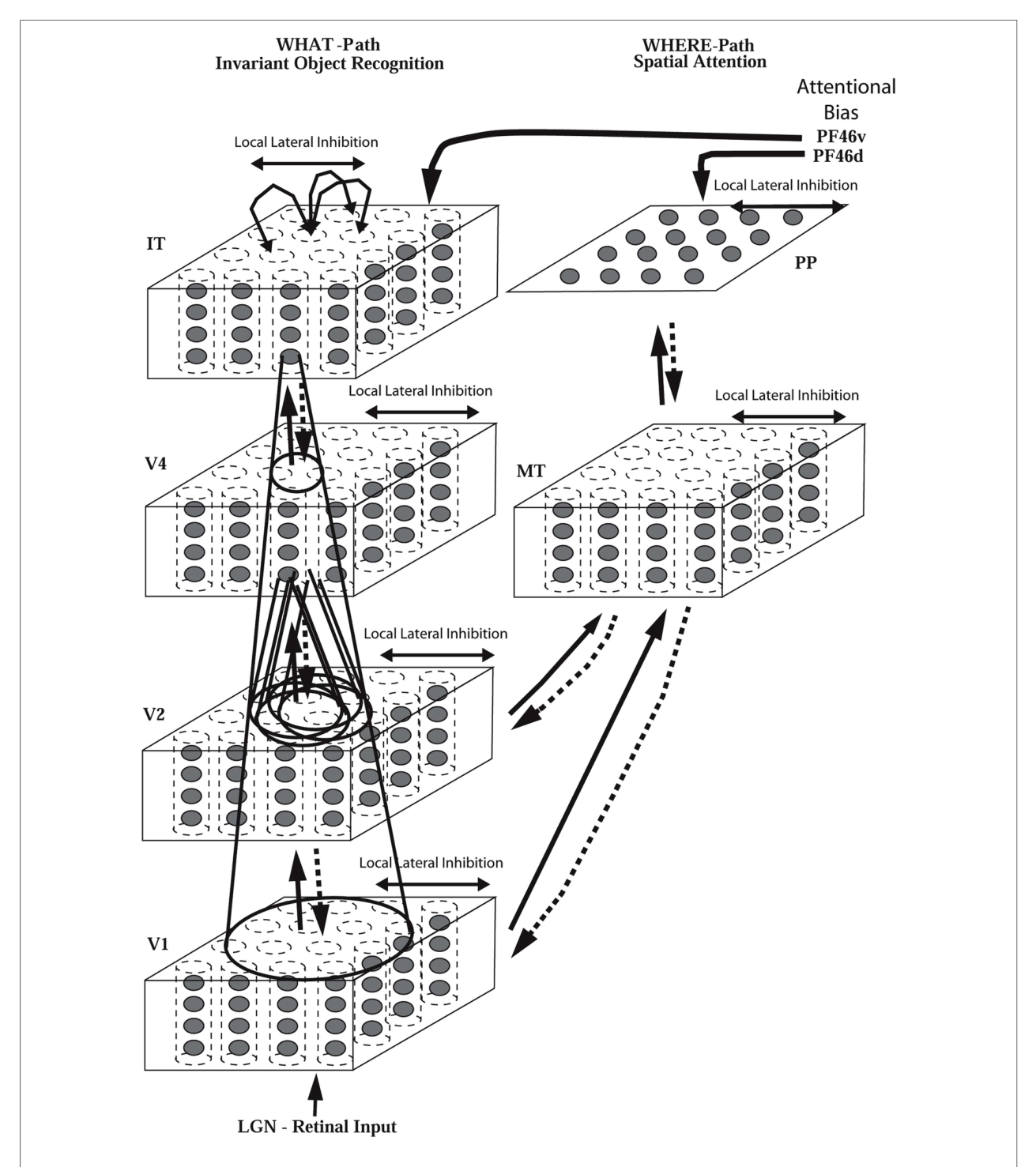
解读:五个模块对应两条通路:腹侧 V1–V2–V4–IT 负责物体识别,背侧 V1→后顶叶(PP)维护物体位置的空间地图;实线为前馈、虚线为自上而下反馈,前额叶 PF46 短时记忆系统对物体流或空间流施加注意偏置。这是把 VisNet 式层级与偏置竞争注意机制整合后的完整架构。
图 35 · 五物体同时呈现时的感受野不对称
原文图注:FIGURE 35 | (A) The responses (firing rate with the spontaneous rate subtracted, means ± sem) of an inferior temporal cortex neuron when tested with 5 stimuli simultaneously present in the close (10°) configuration with the parafoveal stimuli located 10° from the fovea. (B) The responses of the same neuron when only the effective stimulus was presented in each position. The firing rate for each position is that when the effective stimulus (in this case the hand) for the neuron was in that position. The p value is that from the ANOVA calculated over the four parafoveal positions. (After Aggelopoulos and Rolls, 2005.)
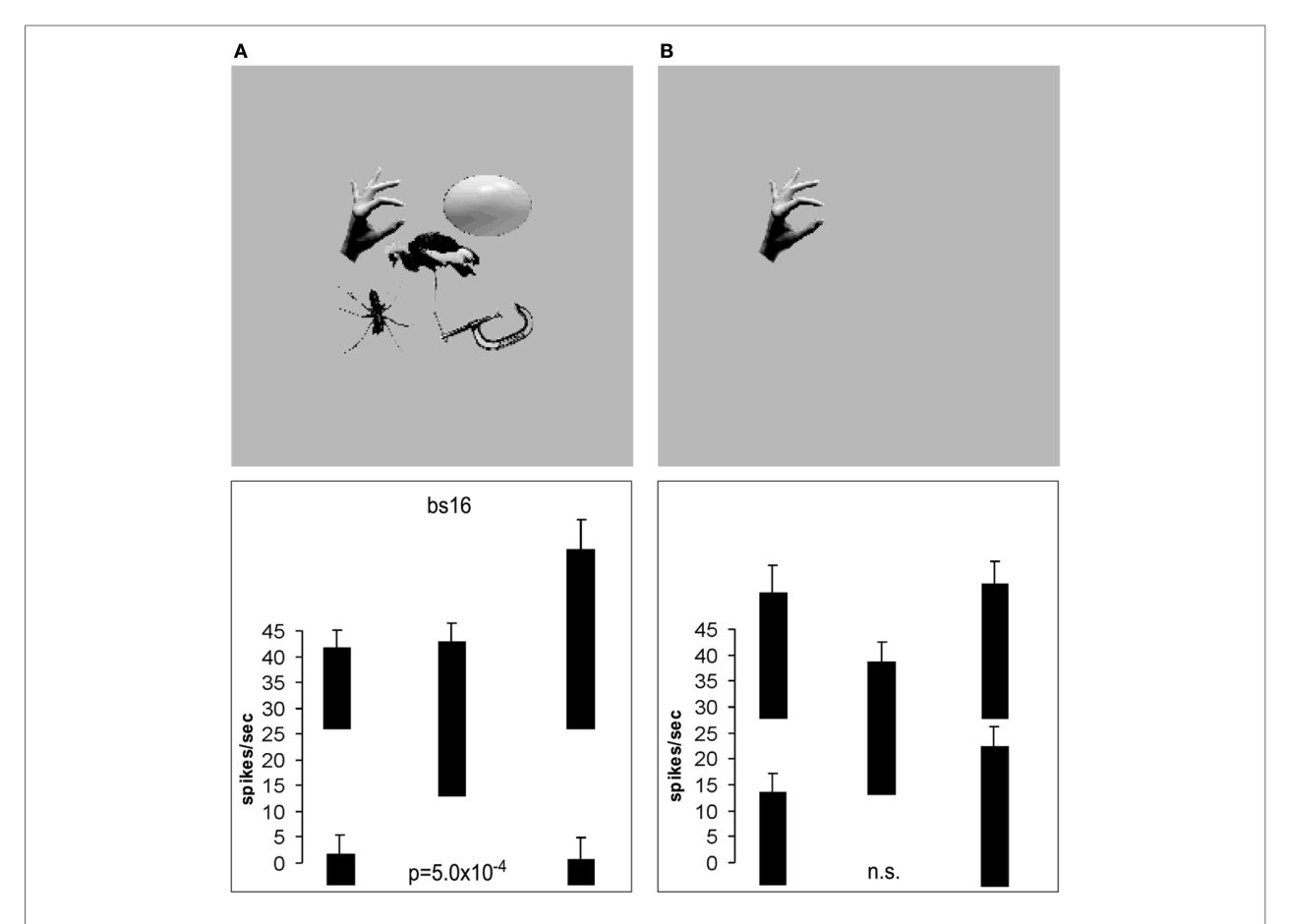
解读:(A) 五个刺激同时呈现(旁中央凹刺激距中央凹 10°)时该神经元(有效刺激是手)在各位置的响应;(B) 只呈现有效刺激时的响应,p 值来自四个旁中央凹位置的 ANOVA。五物体场景中位置间差异显著(感受野不对称被竞争揭示),单刺激时则不明显。这解释了单次注视如何既编码注视物、又携带其他物体的相对位置信息。
图 36 · 连续空间变换(CT)学习
原文图注:FIGURE 36 | An illustration of how continuous spatial transformation (CT) learning would function in a network with a single-layer of forward synaptic connections between an input layer of neurons and an output layer. Initially the forward synaptic weights are set to random values. The top part (A) shows the initial presentation of a stimulus to the network in position 1. Activation from the (shaded) active input cells is transmitted through the initially random forward connections to stimulate the cells in the output layer. The shaded cell in the output layer wins the competition in that layer. The weights from the active input cells to the active output neuron are then strengthened using an associative learning rule. The bottom part (B) shows what happens after the stimulus is shifted by a small amount to a new partially overlapping position 2. As some of the active input cells are the same as those that were active when the stimulus was presented in position 1, the same output cell is driven by these previously strengthened afferents to win the competition again. The rightmost shaded input cell activated by the stimulus in position 2, which was inactive when the stimulus was in position 1, now has its connection to the active output cell strengthened (denoted by the dashed line). Thus the same neuron in the output layer has learned to respond to the two input patterns that have similar vector elements in common. As can be seen, the process can be continued for subsequent shifts, provided that a sufficient proportion of input cells stay active between individual shifts. (After Stringer et al., 2006.)
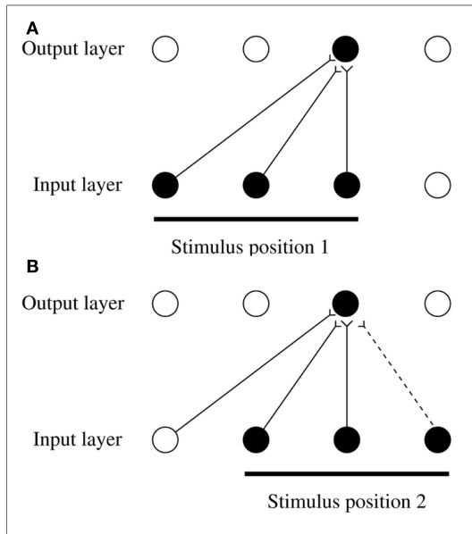
解读:CT 学习的机制图:(A) 刺激在位置 1 时激活的输入细胞经随机前馈连接驱动某输出细胞胜出,其连接被联想规则增强;(B) 刺激小幅移动到部分重叠的位置 2,旧连接足以让同一输出细胞再次胜出,新激活的输入连接(虚线)也被加强。如此沿连续平移逐步"接管",不需要时间痕迹、不依赖呈现顺序——是 trace 学习之外的另一条纯联想路线。
图 37 · 光照不变性
原文图注:FIGURE 37 | Lighting invariance. VisNet was trained on a set of 3D objects (cube, tetrahedron, octahedron, and torus) generated with OpenGL in which for training the objects had left lighting, and for testing the objects had right lighting. Just one view of each object is shown in the Figure, but for training and testing 180 views of each object separated by 1° were used. (After Rolls and Stringer, 2006.)
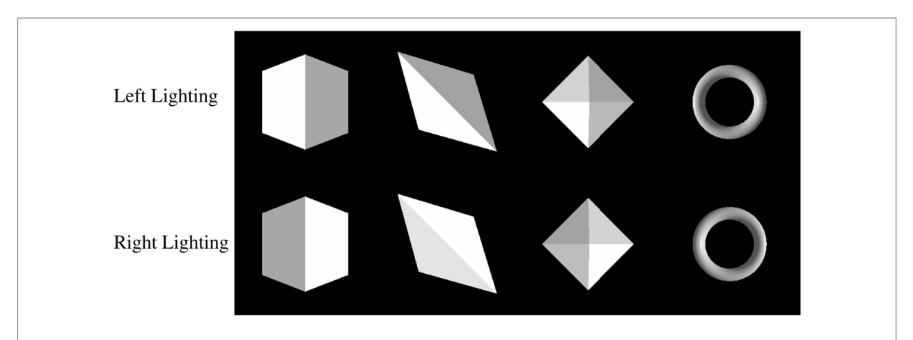
解读:四个 OpenGL 生成的 3D 物体(立方体、四面体、八面体、圆环),训练用左光照、测试用右光照(图中每物体仅示一个视角,实际每物体 180 个 1° 间隔视角)。光照改变后网络仍能正确识别——可能得益于分布式表征保留了跨光照稳定的轮廓类特征,说明 trace 学习的适用范围延伸到光照变换。
图 38 · 背侧通路的全局运动不变性
原文图注:FIGURE 38 | (A) Two rotating wheels at different locations rotating in opposite directions. The local flow field is ambiguous. Clockwise or counterclockwise rotation can only be diagnosed by a global flow computation, and it is shown how the network is expected to solve the problem to produce position-invariant global motion-sensitive neurons. One rotating wheel is presented at any one time, but the need is to develop a representation of the fact that in the case shown the rotating flow field is always clockwise, independently of the location of the flow field. (B–D) Translation invariance, with training on 9 locations. (B) Single cell information measures showing that some layer 4 neurons have perfect performance of 1 bit (clockwise vs anticlockwise) after training with the trace rule, but not with random initial synaptic weights in the untrained control condition. (C) The multiple cell information measure shows that small groups of neurons have perfect performance. (D) Position invariance illustrated for a single cell from layer 4, which responded only to the clockwise rotation, and for every one of the 9 positions. (E) Size-invariance illustrated for a single cell from layer 4, which after training with three different radii of rotating wheel, responded only to anticlockwise rotation, independently of the size of the rotating wheels. (After Rolls and Stringer, 2007.)
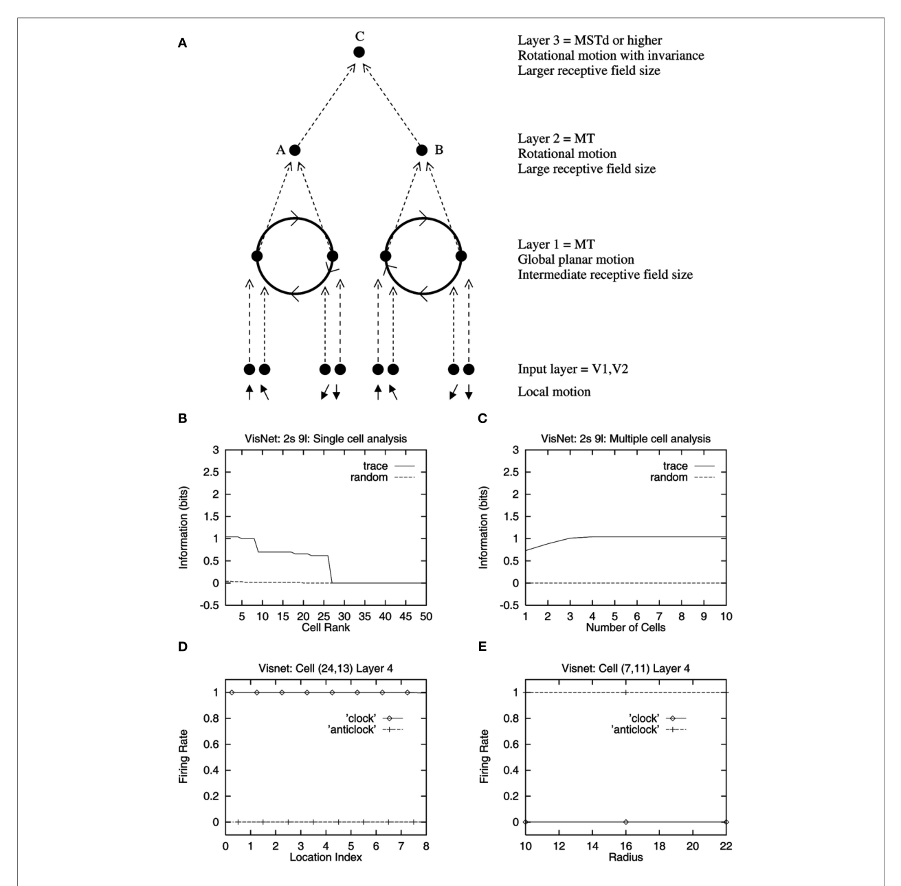
解读:(A) 两个不同位置的旋转轮局部流场等价、旋转方向只能靠全局流计算判定;(B) 9 个位置训练后第 4 层部分神经元单细胞信息达到满分 1 bit(顺 vs 逆时针),未训练对照则不能;(C) 小群神经元的多细胞信息达满值;(D) 一个只对顺时针响应、在全部 9 个位置都响应的单细胞;(E) 用三种半径训练后对尺寸不变。同一 trace 学习原理把腹侧流的结论推广到了背侧流的全局运动表征。
图 39 · 第五层与海马空间表征
原文图注:FIGURE 39 | Adding a fifth layer, corresponding to the parahippocampal gyrus/hippocampal system, after the inferior temporal visual cortex (corresponding to layer 4) may lead to the self-organization of spatial view/place cells in layer 5 when whole scenes are presented (see text). Convergence in the visual system is shown in the earlier layers. Right – as it occurs in the brain. V1, visual cortex area V1; TEO, posterior inferior temporal cortex; TE, inferior temporal cortex (IT). Left – as implemented in VisNet (layers 1–4). Convergence through the network is designed to provide fourth layer neurons with information from across the entire input retina.
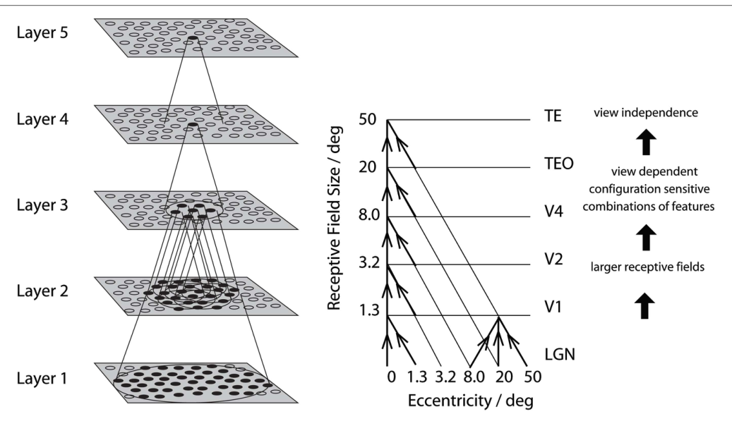
解读:在 IT(第 4 层)之上再加一层对应海马旁回/海马系统的第五层:以整场景(固定相对位置的一组物体)训练时,第五层自组织出对特定场景响应、对同组物体重排出的新场景不响应的神经元——即 spatial view 细胞(灵长类,视野窄)或 place 细胞(大鼠,视野宽)。物体表征与空间表征由此被统一到同一套会聚竞争原理下。
图 40 · HMAX 模型结构
原文图注:FIGURE 40 | Sketch of Riesenhuber and Poggio's (1999a,b) model of invariant object recognition. The model includes layers of "S" cells which perform template matching (solid lines), and "C" cells (solid lines) which pool information by a non-linear MAX function to achieve invariance (see text). (After Riesenhuber and Poggio, 1999a,b.)
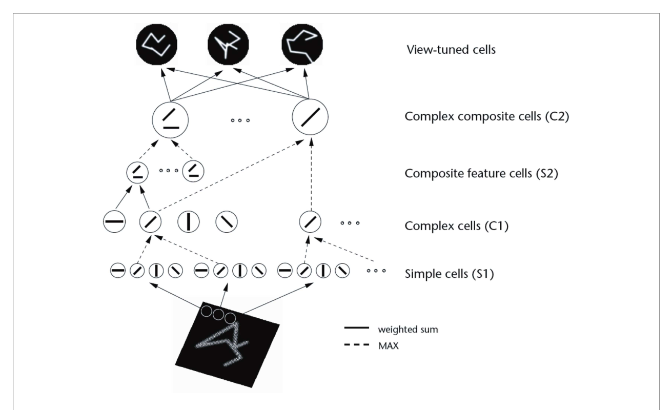
解读:HMAX 的示意:S 细胞层做模板匹配构建更复杂特征,C 细胞层用非线性 MAX 函数池化实现不变性,交替堆叠。它同样是特征层级路线,但架构中不含学习、不变性靠 MAX 池化"内隐扫描"实现,最终输出交由支持向量机分类——与 VisNet 的自组织 trace 学习形成对照。
图 41 · Caltech-256 示例图像
原文图注:FIGURE 41 | Example images from the Caltech-256 database for two object classes, teddy-bears and cowboy-hats.
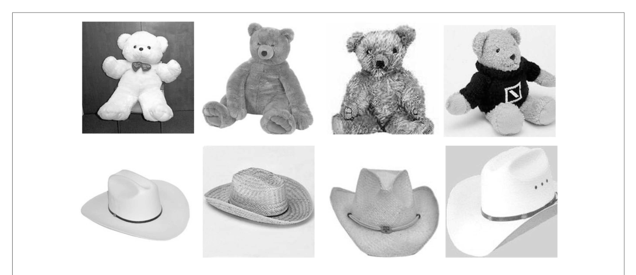
解读:Caltech-256 中泰迪熊与牛仔帽两类的示例图像。该数据库 256 个物体类、类内样本的姿态/光照/尺度/遮挡差异大,来自网络搜集——正是这种类内"不连续性"让后文得出"它不适合训练不变表征"的结论。
图 42 · ALOI 示例图像
原文图注:FIGURE 42 | Example images from the two object classes within the ALOI database, (A) 90 (rubber duck) and (B) 93 (black shoe). Only the 45° increments are shown.
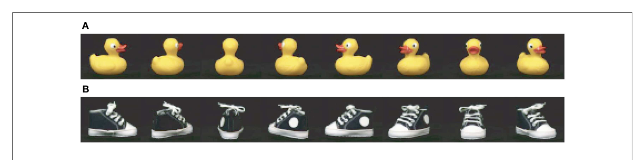
解读:ALOI 数据库的两个类:90 号橡皮鸭与 93 号黑鞋(图中仅示 45° 增量,实际每类 72 张、5° 增量覆盖 360° 旋转)。与 Caltech-256 不同,ALOI 的图像按视角系统变化且相邻连续,为 trace 学习提供了"同一物体的连续变换序列",是检验视角不变学习的合适素材。
图 43 · Caltech-256 上的性能对比
原文图注:FIGURE 43 | Performance of VisNetL, HMAX, and HMAX_min on the classification task using the Caltech-256 dataset. The error bars show the standard error of the means over 5 cross-validation trials with different images chosen at random for the training set on each trial. It is clear that VisNetL performs better than HMAX_min, and this was confirmed statistically using the Chi-square test performed with 30 training images and 30 cross-validation test images in each of two categories (Chi-square = 8.09, df = 1, p = 0.0025).
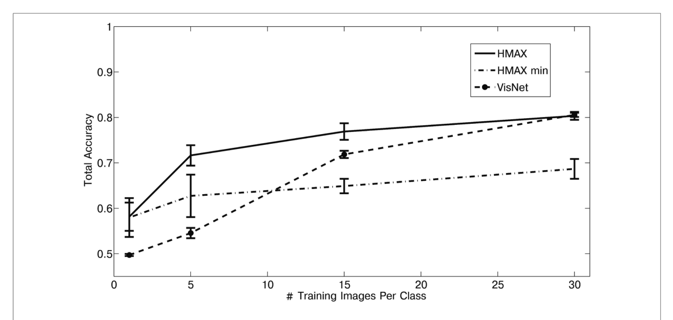
解读:两类任务(泰迪熊 vs 牛仔帽,各 60 张图,训练集 1/5/15/30 张,5 次交叉验证,误差线为均值标准误)下三个模型的分类性能。VisNetL(65,536 神经元)只要有足量训练图就稳定优于 HMAX_min(卡方 8.09,p = 0.0025),完整 HMAX(约千万计算单元)如预期最高——因为它的容量大了百倍以上。
图 44 · ALOI 上的性能对比
原文图注:FIGURE 44 | Performance of VisNetL, HMAX_min, and HMAX on the classification task with 8 classes using the Amsterdam Library of Images dataset. It is clear that VisNetL performs better than HMAX_min, and this was confirmed statistically using the Chi-square test performed with 18 training images 20° apart in view and 54 cross-validation testing images 5° apart in each of eight categories (Chi-square = 110.58, df = 1, p = 10−3).
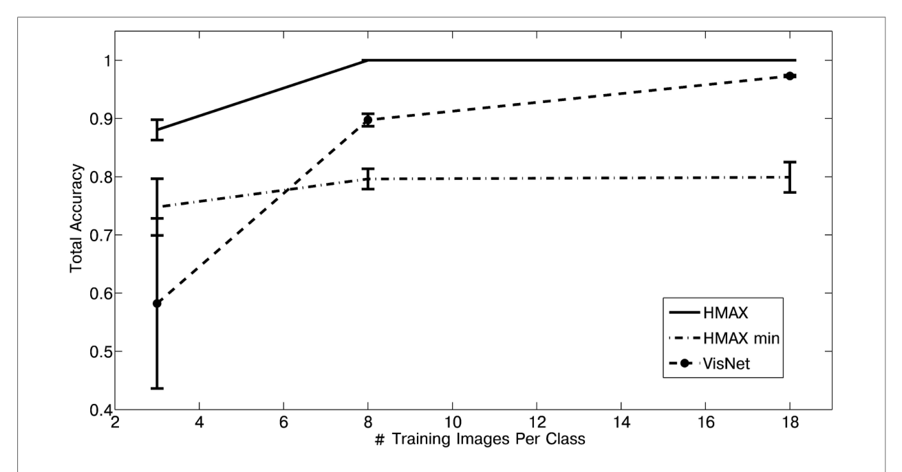
解读:8 个 ALOI 类上的分类性能(18 张 20° 间隔训练图、54 张 5° 间隔测试图,卡方 110.58,p = 10⁻³)。VisNetL 几乎追平大得多的 HMAX;最亮眼的数字是:仅用 45° 间隔的 8 张训练图,就能对距最近训练视角 22.5° 的测试视角保持合理识别——视角采样不必密集。另有一层内对比:ALOI 上第 2/3/4 层分别为 72%/84%/86%(p < 0.001),而 Caltech-256 上各层无差异,反过来证明"训练集必须连续"。
讨论
Rolls 在讨论层面的立场可以概括为三组对照。对"结构描述/语法绑定"路线(图 8)与"同步发放绑定"假说,他以信息论数据反驳:IT 区 94–99% 的信息在发放率中,刺激依赖同步携带不足 5%,且同步本身不指明特征的空间关系,还要追加组合性绑定导致爆炸;VisNet 的方案是让空间语法在学习时"硬编码"进低阶特征组合神经元,运行时不需要任意绑定。对 HMAX(图 40),他承认层级化是"趋同的思路",但指出 HMAX 无学习、MAX 池化缺生物实现、且用 SVM 读出属于另一范式;基准测试的结果反过来引出本文最有分量的方法论结论——Caltech-256 这类类内不连续的数据库根本不适合训练(而非仅仅测试)不变表征,ALOI 这类连续变化的数据库才是正确工具。对容量问题,吸引子分析(图 27–29)给出解析答案:可存物体数与每神经元循环连接数成正比、除以每物体视角数(Po = kC/s),且稀疏编码有利。
文章的局限作者自己也承认:VisNet 模拟的仍是"中央凹小块视野",边界靠环面绕接人工处理;trace 时窗的最优值随层级应不同(早期应短或不启用)这一主张虽有推理但未逐一验证;将其标为解读者推论,或只陈述“半数视角训练、其余视角交叉验证时约为68%正确率;作者认为表现合理,并指出进一步扩展容量仍需研究”。;与真实神经生理的对应(如痕迹的生物学基础——NMDA 受体、持续放电、一氧化氮等)仍属候选机制而非定论。文中未详述的部分包括模型与人脑 fMRI 数据的定量对接,以及跨物体连续性的容量极限。总体上,他把"不变表征"的账算给了一个统一原理:层级会聚 + 竞争 + 利用世界时空统计的局部可塑性学习——同一原理覆盖腹侧流、背侧流与海马。
一句话总结
在我看来,这篇综述的真正贡献是把"不变性从哪里来"这个问题从工程 tricks 还原成了一个可以逐条检验的神经科学命题:物体在时空中的连续性本身就是监督信号,而皮层只需要会聚、竞争和一个带 0.5 秒记忆的 Hebb 规则。trace 规则"比随机还差"的纯 Hebb 对照是我印象最深的实验设计——它说明不变性学习的要点不是"增强同时出现的连接",而是"增强刚刚出现过它的那个东西现在的连接"。文中对基准数据库(Caltech-256)的批评在今天深度学习时代读来仍有先见之明,只是当时没有 ImageNet 式的连续变换数据来彻底检验它,这是我作为读者的判断。
审校与证据追溯 (Verification & Evidence)
图表审计结果
- Fig1: 提取质量
good,对齐度full,识别面板[] - Fig10: 提取质量
good,对齐度full,识别面板[] - Fig11: 提取质量
good,对齐度full,识别面板[] - Fig12: 提取质量
good,对齐度full,识别面板[] - Fig13: 提取质量
good,对齐度full,识别面板[] - Fig14: 提取质量
good,对齐度full,识别面板[] - Fig15: 提取质量
good,对齐度full,识别面板[] - Fig16: 提取质量
good,对齐度full,识别面板[] - Fig17: 提取质量
good,对齐度full,识别面板[] - Fig18: 提取质量
good,对齐度full,识别面板[] - Fig19: 提取质量
good,对齐度full,识别面板[B] - Fig2: 提取质量
good,对齐度full,识别面板[] - Fig20: 提取质量
good,对齐度full,识别面板[A, B, C] - Fig21: 提取质量
good,对齐度full,识别面板[] - Fig22: 提取质量
good,对齐度full,识别面板[] - Fig23: 提取质量
good,对齐度full,识别面板[] - Fig24: 提取质量
good,对齐度full,识别面板[A, B, C] - Fig25: 提取质量
good,对齐度full,识别面板[] - Fig26: 提取质量
good,对齐度full,识别面板[A] - Fig27: 提取质量
good,对齐度full,识别面板[] - Fig28: 提取质量
good,对齐度full,识别面板[A] - Fig29: 提取质量
good,对齐度full,识别面板[A] - Fig3: 提取质量
good,对齐度full,识别面板[] - Fig30: 提取质量
good,对齐度full,识别面板[] - Fig31: 提取质量
good,对齐度full,识别面板[] - Fig32: 提取质量
good,对齐度full,识别面板[] - Fig33: 提取质量
good,对齐度full,识别面板[A, B] - Fig34: 提取质量
good,对齐度full,识别面板[] - Fig35: 提取质量
good,对齐度full,识别面板[A, B] - Fig36: 提取质量
good,对齐度full,识别面板[A, B] - Fig37: 提取质量
good,对齐度full,识别面板[] - Fig38: 提取质量
good,对齐度full,识别面板[A, B, D] - Fig39: 提取质量
good,对齐度full,识别面板[] - Fig4: 提取质量
good,对齐度full,识别面板[] - Fig40: 提取质量
good,对齐度full,识别面板[] - Fig41: 提取质量
good,对齐度full,识别面板[] - Fig42: 提取质量
good,对齐度full,识别面板[A, B] - Fig43: 提取质量
good,对齐度full,识别面板[] - Fig44: 提取质量
good,对齐度full,识别面板[] - Fig5: 提取质量
good,对齐度full,识别面板[] - Fig6: 提取质量
good,对齐度full,识别面板[] - Fig7: 提取质量
good,对齐度full,识别面板[A] - Fig8: 提取质量
good,对齐度full,识别面板[A] - Fig9: 提取质量
good,对齐度full,识别面板[]
关键事实与局限性声明
- 审校纠偏: {'classification': 'OVERCLAIM', 'md_section': '图39;主要结果', 'current_text': '加第五层可自组织出海马 spatial view/place 细胞', 'problem': '把场景特异模拟结果扩大成已经验证的spatial-view/place细胞形成机制。', 'recommended_fix': '降级为作者提出并部分模拟支持的计算假说。'} -> 评注:
- 审校纠偏: {'classification': 'OVERCLAIM', 'md_section': '图44;讨论', 'current_text': 'Caltech-256上各层无差异,反过来证明“训练集必须连续”;Caltech-256根本不适合训练不变表征,ALOI才是正确工具', 'problem': '原文结果仅直接支持VisNetL及这类依赖连续性学习的会聚层级模型。它不能普遍证明所有不变识别系统的训练集都必须连续,也不能确立ALOI是唯一“正确工具”。', 'recommended_fix': '改为“在VisNetL及类似依赖时空连续性的模型中,Caltech-256类内样本不足以支持有效的trace学习,而ALOI的连续视角变化更适合作为训练数据”。'} -> 评注:
- 审校纠偏: {'classification': 'OVERCLAIM', 'md_section': '一句话总结', 'current_text': '皮层只需要会聚、竞争和一个带0.5秒记忆的Hebb规则', 'problem': '模拟表明这些机制在特定架构和训练条件下具有计算可行性,但没有在脑内建立必要性、充分性或因果机制。NMDA受体、持续放电和一氧化氮仅是候选生物实现。', 'recommended_fix': '改为“作者提出,会聚、竞争和约0.5秒的活动痕迹可能构成学习不变表征的一组可行机制”。'} -> 评注:
- 补充要点: 本文没有统一样本量;必须将综述所引既往实验与本文自身的计算模拟分开。
- 补充要点: Booth和Rolls的熟悉物体研究包含10个在猴笼中暴露数周的真实塑料物体,以及从未作为真实物体见过的控制物体视图。
- 补充要点: 杂乱背景学习失败不仅提示可能需要分割;原文还指出固定背景使神经元容易学习背景而非目标,是该负结果的重要技术原因。
- 补充要点: 部分遮挡实验在空白背景下进行,以避免把遮挡效应与背景杂乱混淆。
- 补充要点: 第五层场景模拟验证的是场景及相对空间关系选择性;窄视野spatial-view细胞与宽视野place细胞的分化仍是未来检验项目。