IT Literature Intelligence 终审版本 (VERIFIED) 论文编号:
214| 原始基线:V0_ZCODE_BASELINE| 语义审核:needs_revision| 图表审核:minor_issue
Learning to Recognize Visual Objects With Microstimulation in Inferior Temporal Cortex
Kawasaki · Journal of Neurophysiology · 2008 · Zotero itemID=2032
这篇文章直接回答"IT(下颞叶,inferior temporal cortex)活动是否足以支撑视觉联结学习"这个充分性问题:在猴子学习给新图形分类的同时,对 IT 做局部微刺激,让电流本身充当分类线索。结果显示微刺激确实可以用来"教会"分类,学习后的同一刺激还会系统性地偏置对全新混合图形的判断,而这种效应换到邻近听觉区就失效。它值得读在于用一种少见的"电流当线索"设计,把相关证据(学习改变 IT 选择性、IT 损伤削弱学习)补成了一条因果链。
研究背景
猕猴 IT 是腹侧视觉通路的最高级区域之一,神经元选择性响应特定物体特征及其组合(Desimone et al. 1984; Tanaka et al. 1991),既接收来自早期视觉区的前馈输入,也接收内侧颞叶结构和前额叶的反馈。以往研究为"IT 在视觉联结学习中起关键作用"提供过两条证据:一是相关性——学习会改变 IT 神经元的选择性(视觉-视觉联结、视觉-运动联结、视觉-奖励联结,Sakai & Miyashita 1991; Kobatake et al. 1998; Mogami & Tanaka 2006 等);二是必要性——IT 功能失活会破坏已建立的视觉辨别并增加学习新辨别的试次(Brown & Schafer 1888; Chow 1961; Horel 1996 等)。但"当下的 IT 差异活动是否足以建立新联结"一直没有正面答案,因为相关研究无法制造、失活研究只能去除活动。
同时,脑刺激文献里有两条可参照的线索与陷阱。Doty 等(1965, 1964)用大电流表面电极把皮层刺激当成条件刺激教会猴子回避,刺激本身可引出条件反应;近年 Romo 等(2000,S1)、Salzman 等(1992,MT)的微刺激研究都假定"预先存在的功能组装"可以被定向激活。本文要做的对象表征学习与这些都不一样:被学习的模式是猴子从未见过的,刺激位点也没有按选择性挑选。
研究思路
作者的总体逻辑是把"IT 微刺激在信息量梯度上的作用"逐级拆开,每一级排除一类替代解释。第一级,"刺激信息是排他的"(exclusively informative):一个视觉图形同时映射到左右两个按钮,正确按键只取决于呈现时 IT 有没有通电——如果差异活动足以支持学习,猴子应该学会利用它。第二级排除"直接把刺激跟运动绑定"的解释:插入纯刺激试次(无视觉图形)看会不会按键;再让第二个新模糊图形沿用相反的映射,看学习是否依赖具体图形。第三级,"刺激信息是条件性的"(conditionally informative):模糊图形永远伴随固定的 200 ms 电刺激序列,判别的唯一线索是电与视觉的相对时序(视觉前 vs 视觉中)——此时"有没有刺激"本身不再有用。第四级,"刺激信息有用但不必要"(informative but not necessary):学习期四个图形之一始终伴随刺激,之后引入图像混合技术合成的新图形,看刺激是否按训练时的绑定方向偏置选择;再对比含/不含配对图形的混合来检验特异性。外部对照链则问:换一个真实的听觉线索行不行?把刺激从 IT 挪到邻近的听觉反应区行不行?
方法
三只恒河猴(8–11 kg),头部固定,记录室植入在一侧半球(立体坐标 AP 17 mm、ML 20 mm,提供进入颞叶皮层的垂直通道)。钨微电极(阻抗 250 kΩ–1.0 MΩ)借液压微推进器进入前下颞叶,以在线多单位视觉响应直方图选定视觉反应位;沿电极轨迹的灰白质模式与立体坐标把位点估定在细胞构筑区 TE 附近(ventral area 36 外侧、TEO 之前)。刺激由模拟刺激隔离器加可编程波形发生器输出,双相脉冲 200 Hz、脉宽 200 µs,不锈钢导引管作返回通路,串联 1 kΩ 电阻并用电池供电放大器对实际电流永久记录。视觉刺激呈现在 22 英寸 CRT 上(刷新 100 Hz,观察距离 119 cm),眼位用高速红外摄像机(EyeLink II)监测;行为与计时由 QNX 实时操作系统控制的 PC 网络管理。任务结构四种:1)消歧任务——每会话 3 张新图像(乌克兰彩蛋),两张分属左右键(distinct),第三张同图两键皆可、正确映射仅取决于 IT 电刺激有无(ambiguous),视觉与电刺激时长均为约 1 s(若提前按键则两者同时中止);2)相对时序任务——视觉 200 ms,模糊图形永远伴 200 ms 刺激序列,一半试次刺激先于视觉 200 ms、一半在视觉出现 75 ms 后开始,且视觉/电序绝对时刻随机化,参数为 30 或 60 µA;3)脑区特异性——用一只熟悉分类任务但从未受过微刺激消歧训练的猴,隔日交替在 IT(75 µA)与邻近听觉区(LFP 定位,距 IT 约 6 mm、更浅、邻近 TPO/TAa)各做 400 试次,重复 10 轮;4)泛化任务——每会话 4 张新邮票图,2 张直立、2 张旋转 45 度,直立之一全程搭配 200 ms、30 µA 刺激(视觉出现后 75–275 ms),每图学习 100 次;之后用透明度(alpha 通道)混合两图合成新刺激,先以固定比例预试并用 logistic 函数估出主观中点,再取中点附近预计产生 30/50/70% 右反应的三个混合比测试,模糊刺激不论选择按 75% 概率奖励。分析上,学习效应看每条件最后 48 试次(二项检验),选择偏移用刺激系数的 logistic 回归(似然比检验)与每猴 Wilcoxon 符号秩检验,反应时用双向方差分析(刺激×选择),首扫视端点用 ROC 曲线下面积量化眼动分离。
主要结果
- IT 微刺激足以消歧同一视觉图形:24 次实验(S、J 各 12 次,刺激侧随机)中 21 次出现显著学习(P<0.05,二项检验);模糊条件平均正确率 79%(S 82%、J 76%),而 distinct 对照高达 98%。distinct 条件约 10 次重复即达 80% 正确,ambiguous 条件更慢;各会话学习速率没有变快,无"学会学习"迹象(图 1)。
- 排除两个替代解释:在 5 个成绩达 80% 的会话里混入 4/32 纯电刺激试次(无视觉图形),两只猴都等满 5 s 超时不作反应,说明刺激本身单独不足以触发反应;眼动上,distinct 条件首扫视轨迹按图形明显分离,ambiguous 条件则无清晰分离,扫视端点 ROC 分离与成绩的相关只在猴 J 后期出现(r=0.58, P=0.05)——作者结论眼动分离是学习后的反应规划结果而非学习的信息来源(图 2)。
- 相对时序可学,且强度依赖——排除"存在检测"解释:模糊图形固定配 200 ms 刺激、仅"电先于视觉"或"电迟于视觉 75 ms"区分左右时,30 µA 下 12 次实验 4 次显著(33%),电流翻倍至 60 µA 后 13 次中 10 次显著(77%)。猴子用相对时序判别,说明"检测到刺激"不是唯一可用信息(图 3)。
- 效应脑区特异、换听觉线索则失效:把模糊线索换成与视觉同步的真实世界声音(70–74 dB SPL),同样的猴子 14 次实验(S 6、T 8)无一显著学习(平均 49%),尽管定向测试证实它们听得见(声源朝向 79% 与 80%);隔日交替训练中,IT 刺激 10 次里 8 次显著(平均 68±12%)、听觉区刺激仅 1 次显著(69%,平均 52±6%),两群体差异 P<0.001(Wilcoxon 秩和检验)(图 1D、图 4)。
- 学习后的电流信号可预测地偏置对新混合图形的选择,且偏置带刺激特异性:logistic 回归的刺激系数,含配对图形的混合为 S 0.67、T 0.31(均 P<0.001,似然比检验),不含配对图形的(旋转混合)仅 S 0.2(P<0.05)、T 0.09(n.s.);效应量从 11.0% 降到 3.5%(转移下降 68%,P<0.001,Wilcoxon 符号秩检验),而配对混合上的偏置本身在两猴均显著(Wilcoxon 符号秩检验,均 P<0.05)。反应时同步变化:加电后选择"预测"侧更快、选"非预测"侧更慢(S P<0.001、T P<0.01),不含配对图形的混合无反应时效应(图 5–8)。
图注解读
图 1 · 用 IT 电刺激消歧图形:任务、学习曲线与听觉对照
原文图注:FIG. 1. Electrical stimulation in inferior temporal cortex (IT) to disambiguate visual patterns. A: single trial in the basic discrimination task consisted of the presentation of a fixation square followed by a visual stimulus for ±1 s, the monkey's response (left or right button press), and a feedback signal (tone, plus juice reward on correct trials). B: for each session in this experiment, 3 novel images of painted Ukrainian eggs were selected and mapped to button responses as shown. Two of the 3 images were unique and assigned to the left and right buttons (distinct). The 3rd image was assigned to both the left and right buttons and could only be distinguished by accounting for the presence or absence of the electrical stimulation (ambiguous). During the experiment, the 4 stimuli were randomly interleaved on separated trials. C: learning curves for 3 sessions (top and middle rows are from microstimulation sessions, bottom row is from an auditory stimulation session), comparing performance for trials containing the 2 distinct stimuli (left) and the 2 visually ambiguous stimuli (right). Learning in the distinct condition required 10 stimulus repetitions to achieve 80% correct performance. In the ambiguous condition, learning proceeded more slowly. The side assigned for ambiguous plus electrical stimulation is denoted on the top of plots. In 1 experiment (middle row), we introduced a 2nd ambiguous set (indicated by a gray vertical line) after learning of the 1st set was complete. The response mapping for the second ambiguous plus stimulation pair was reversed. In this case, the monkey showed a chance level performance for initial trials and proceeded to learn the new mapping without interference from or interfering with performance on the already learned stimuli. D: comparing the effects of electrical microstimulation with auditory stimulation. Bars show average performance for the last 48 trials in conditions where stimuli could be distinguished based on visual differences (Visual/Visual), on the presence or absence of electrical microstimulation (Visual/IT microstimulation), and on the presence or absence of auditory signals (Visual/Auditory). Each circle represents performance from each experiment. Filled circle, session showed significant learning effects; open circle, no significant learning. Performance in the electrical microstimulation condition was clearly superior to that in the auditory condition, showing that integration of disambiguating information does not always occur. Error bars denote SD.
解读:A、B 是任务与映射规则,关键在 ambiguous 图形——同一张图在"带电"与"不带电"试次里分别该按不同的键。C 左右两列分别是 distinct 与 ambiguous 条件的学习曲线:distinct 很快到 80%,ambiguous 慢得多;中行的灰线之后还引入了第二个 ambiguous 集、映射反转,猴子从机会水平重新学起而旧的对子不受牵连。D 的柱状比较里,Visual/Visual 与 Visual/IT microstimulation 两种条件整体在高水平(ambiguous 条件多数实验显著学习),Visual/Auditory 一支大多空开、均值近 49%。这张图支撑结果 1、2 与 4 的前半部分。
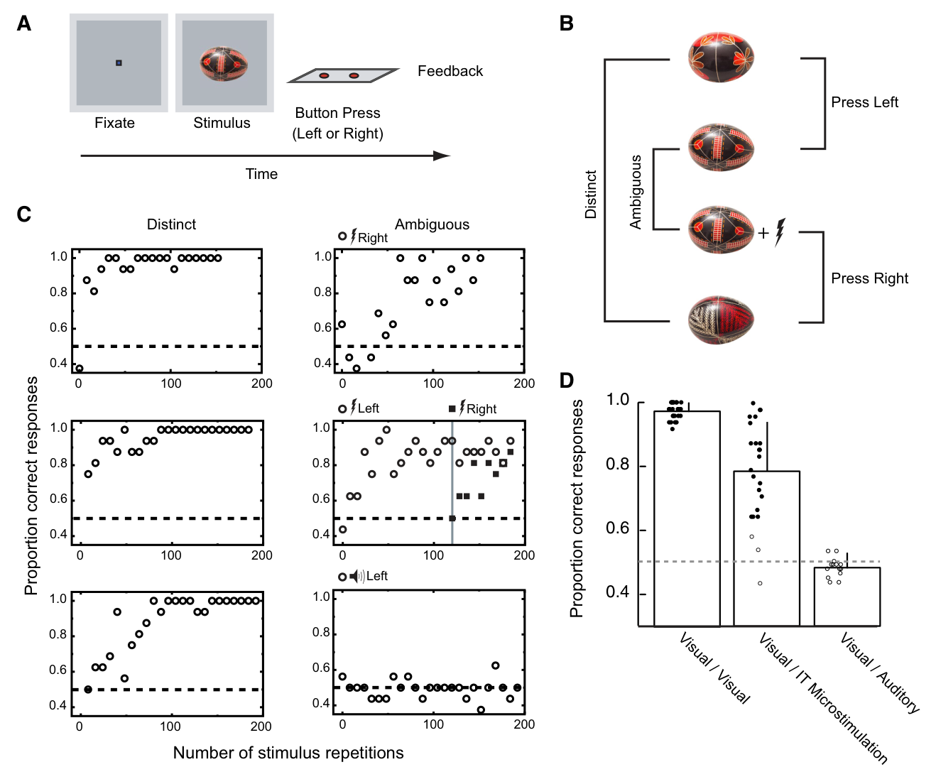
图 2 · 首扫视对照:眼动分离不解释学习
原文图注:FIG. 2. Initial saccades in the distinct and ambiguous conditions. A: initial saccade trajectory and histograms of saccade endpoints from individual sessions. Positive value in horizontal and vertical eye displacement indicates displacement to the right and up, respectively. Top row: data from monkey S. For a distinct visual stimulus pair (top left panel), saccades for one stimulus, which was assigned to left button pressing (trajectory and histogram shown in black), and another stimulus, which was assigned to right button pressing (trajectory and histogram shown in green), showed a segregated trajectory. Stimuli used for each condition is inset left above of the trajectory panel. For an ambiguous pair (top right panel), saccades showed similar overall profile but no clear separation between unstimulated condition, which was assigned to left button pressing (trajectory and histogram shown in black), and stimulated condition, which was assigned to right button pressing (trajectory and histogram shown in red). Stimuli used for each condition is inset left above of the trajectory panel. A scatter plot placed under the each eye trajectory panel represents behavioral learning curve from the same session. Another example session from monkey J is shown on bottom row. In this case, stimulated condition (trajectory and histogram shown in red) was assigned to left button pressing. B: eye separation and behavioral performance in the ambiguous condition. Population data from monkey S (12 sessions) and monkey J (12 sessions) are shown in left and right panels. Ordinate (for eye separation) shows area under the curve with receiver operating characteristic (ROC) analysis for endpoint positions in horizontal axis. Abscissa (for behavioral performance) shows mean correct rate at the period that the eye separation is calculated. Each point represents data from 24 trial repetitions. Symbols represent learning phase (periods within each session). Red filled circle indicates initial 24 repetitions at the beginning of each session (early blocks). Pink unfilled square indicates last 24 repetitions of each session (late blocks). Unfilled circle indicates middle phase between initials and lasts (middle blocks).
解读:A 用轨迹与端点直方图并排展示两个条件:distinct 配对下扫视已按图形分流(黑 vs 绿),ambiguous 配对(黑 vs 红)整体分布相似却没有这种分离——即控制眼动位置并不能给猴子提供区分线索。B 把每个 24 试次块的 ROC 面积(眼分离)对同块正确率作散点:猴 S 无相关(r=−0.006, P=0.95),猴 J 整体有相关(r=0.56, P<0.001)但分成早/中/晚块后发现只有后期块显著。合起来支撑结果 2 的最后一句:眼动偏置是学习形成后的伴随品,不是学习的机制。
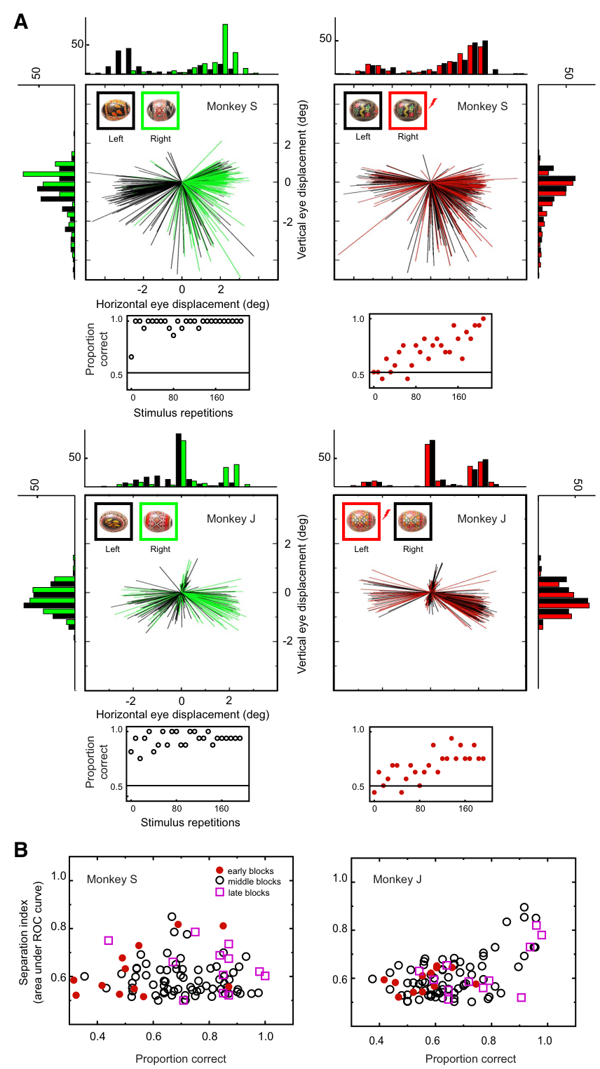
图 3 · 相对时序任务:检测到"有电"还要知道"何时"
原文图注:FIG. 3. Sensitivity to relative timing between electrical and visual stimulation. A: the paradigm was similar to that shown in Fig. 1 except that all visually ambiguous trials included a 200-ms train of electrical stimulation (200 Hz, 200 µs width biphasic pulses). New stimuli and stimulation sites were selected for each experiment session. The relative timing between the onset of the electrical and visual stimulus determined the proper button mapping for each ambiguous pair. B: proportion correct for the final 48 trials is shown for both the visual distinct control stimuli (left 2 columns) and the visual/electrical pairs (middle and right columns). With current levels set to 30 µA (circles), learning was evident in 4/12 experiments (filled symbols). At 60 µA (squares), we observed significantly above chance performance in 10/13 experiments (filled symbols).
解读:A 说明这个变体里,ambiguous 图形每次都带 200 ms 刺激,判别规则只能来自相对时序(stim 先于视觉 vs 迟于视觉 75 ms),且视觉/电的绝对时刻做了随机化,让"刺激在何时出现"本身不可作为答案。B 是末 48 试次的正确率散点:左侧两列 distinct 对照几乎都在 0.8–1.0;中列(30 µA)模糊条件只有 4/12 个实心点(显著学习),右列(60 µA)10/13 个实心点。横跨两列的对比支撑结果 3——提高电流后学习率近乎翻倍,说明该任务可用但更苛刻,排除了"只要能检测到刺激就会做"的解释。
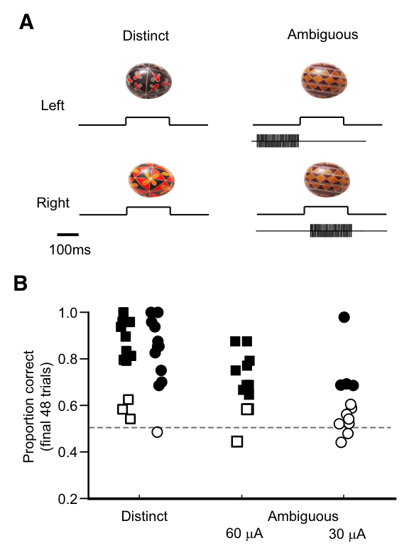
图 4 · 同类学习在听觉区不成立
原文图注:FIG. 4. Areal specificity of learning effects. A, left: depth profile of local field potentials (LFPs). Illustration of the estimated coronal brain section superimposed on LFPs evoked by auditory (green line) and visual (red line) stimuli. Right: an alternate day training schedule was applied to microstimulation learning in a learning naïve monkey to compare learning rates for stimulation in visual and auditory responsive areas. B, left: averaged learning curve from 10 IT stimulation experiments. Performance (y axis) for distinct condition (unfilled circles) and ambiguous condition (filled red circles) is plotted against number of stimulus repetitions. Right: average learning curve from ten auditory area stimulation experiments. Performance (y axis) for distinct condition (unfilled circles) and ambiguous condition (filled green circles) is plotted against number of stimulus repetitions. Error bars denote SD. C, left: averaged LFP from 10 IT stimulation sites. Right: averaged LFP from 10 auditory area stimulation sites. Red line shows response for visual stimuli. Green line shows response for auditory stimuli. x axis represents time after onset of visual and auditory stimulus. Y axis represents amplitude of LFP.
解读:A 左的深度剖面(局部场电位,local field potentials, LFP)说明同一条电极轨迹上可分别找到听觉(绿)与视觉(红)反应层,从而保证对照在"同一条轨道、相距约 6 mm"的两个位点进行。B 左右分别给出 IT 刺激(10 次实验)与听觉区刺激(10 次实验)的平均学习曲线:红实心(IT ambiguous)随重复稳步脱离 distinct 水平并显著(8/10 会话),绿实心(听觉区 ambiguous)基本贴在机会水平附近(仅 1/10 显著)。C 是两个位点群的平均 LFP,验证视觉/听觉选择的定位。这张图支撑结果 4:效应不是"任何皮层电流都行",而是针对 IT。
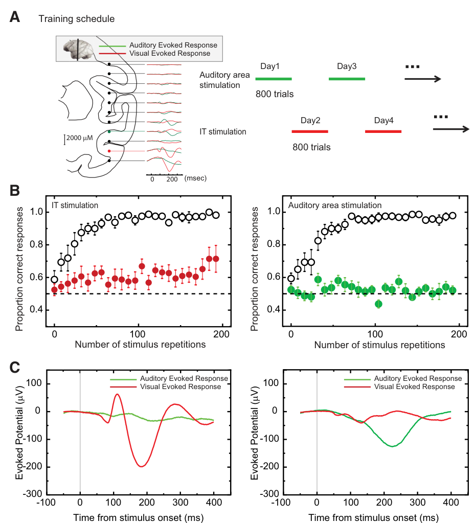
图 5 · 泛化任务设计与学习期对照
原文图注:FIG. 5. The effects of IT microstimulation during visual classification learning when microstimulation is informative, but not required, for classification. A: in this task, 4 new images of stamps were selected before each test session. Random colored noise was added to each stimulus to introduce initial variability during the discrimination task. Two stimuli were shown upright, and 2 were rotated 45°. Microstimulation was included on all trials containing 1 of the 2 upright stimuli (randomly assigned to either the left or right in each session). Thus during learning, 1 of 4 patterns was always experienced with the microstimulation present. Inset: the recorded analog return signal from the stimulating electrode, which verified the timing and amplitude of the microstimulation. The rotated stamps served as control stimuli in each experiment. B: performance plotted as a function of number of stimulus repetitions shows that for this task, the additional microstimulation (filled circles) did not significantly affect learning rates of the patterns assigned to the stimulation condition compared with performance for unstimulated stimuli (open circles). By 100 stimulus repetitions per stimulus, performance was between 90 and 100% for both trial types.
解读:A 交代泛化任务的四张邮票(2 直立、2 旋转)与"只有一个直立图形带刺激"的绑定规则,内插小图是刺激电极回路上记录的模拟信号,证明电流按时按幅送达。B 是学习阶段的对照:带刺激与不带刺激的图形学习曲线重叠,100 次重复后两类都在 90% 以上——本设计里电流对学习速度本身没有附加增益,这与消歧任务(电流是唯一线索)不同,把后面图 7 的偏置效应明确限定为"学习后测试阶段"的现象。
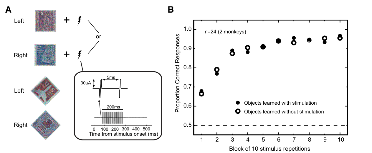
图 6 · 单次实验中的心理测量曲线与电流偏置
原文图注:FIG. 6. The effect of electrical microstimulation on the classification choices for novel stimuli composed of image mixtures. A: psychophysical performance from a single behavioral experiment shows the systematic effect of varying the stimulus content from 100% left stimulus to 100% right stimulus. After a learning phase consisting of 100 repetitions for each of the individual stamps, stimulus blends were created by mixing the 2 stamps from the same orientation condition (upright or rotated) in various proportions. A brief pretest with fixed blend ratios (see METHODS) was administered, and the data were fit to a sigmoid function to estimate the midpoint for response selection (which was not always at the 50% blend level). Three levels of mixing around this subjective midpoint were then used for the main test condition. The abscissa for these plots represents the proportion of the right stimulus at each point, and the ordinate shows the proportion of right responses chosen. At the extremes, the animal's choices were close to perfect and choices between the 2 extremes varied smoothly and systematically as a function of blend proportion. B, left: comparison of stimulated (filled circles) and unstimulated (open circles) trials shows a systematic shift in response proportion upward in the direction of the response associated with the stimulus paired with microstimulation during learning. The microstimulation induced shift was measured as the average response difference between the stimulated and unstimulated conditions in the ambiguous region of the response curve (data appeared on gray background). Right: effect of microstimulation on trials from the same experimental session containing mixtures of images neither of which had been previously been associated with microstimulation. There is transfer of the effect of microstimulation (for this experiment, microstimulation biased choices to favor the right hand response), but the magnitude of this shift was systematically smaller than that observed for the visual mixtures that included the previously associated image (see Fig. 7).
解读:A 给无刺激的基线心理测量曲线——横轴是混合中"右图形"占比,纵轴是选右的比例;两端几乎完美、中间平滑过渡,拐点(主观中点)不一定在 0.5 处,故预试先行估计。B 是关键对比:左图里实心(刺激试次)相对空心(无刺激)在灰底模糊区域内整体上移,方向指向学习期与电流绑定的那个图形;右图是同一会话中不含配对图形的旋转混合,电流也造成偏移但幅度小得多。这张图支撑结果 5 的两条分支:整段偏置存在、偏置又是刺激特异的。
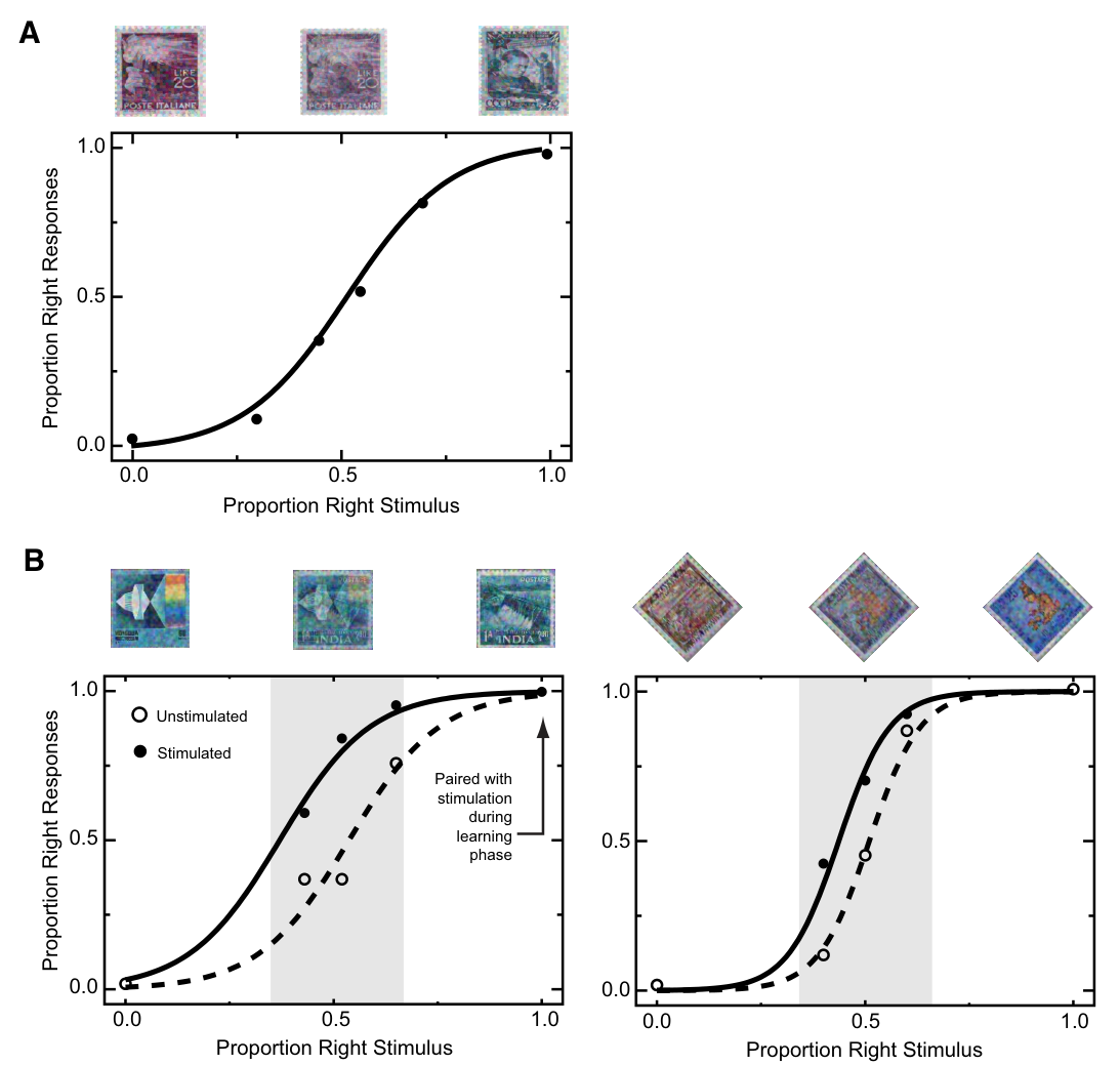
图 7 · 群体效应与特异性的量化
原文图注:FIG. 7. Stimulation induced response shifts and a test of stimulus specificity. A: population plots and psychometric functions from monkey S (12 experiments, top row) and monkey T (12 experiments, bottom row). F and E, responses with and without electrical stimulation, respectively. — and - - -, fitted psychometric functions for trials with and without electrical stimulation. The psychometric function is obtained by logistic regression analysis for the choices made in response to the stimuli mixture containing the image previously been associated with microstimulation (left) and for mixtures wherein neither of the source images had been previously associated with microstimulation (right). B: 24 experiments were conducted in 2 monkeys comparing the response to ambiguous stimulus blends (Fig. 6) with and without stimulation. Effect size (abscissa) is measured in terms of response bias with positive indicating more responses in the direction of the unblended stimulus that had been paired with stimulation during learning. On average, both monkeys showed a significant shift in the expected direction with a mean amplitude across the set of experiments of 11%. C: the specificity of the stimulation effect was assessed by comparing the shift in response bias caused by microstimulation between the blends of upright stamps (which always included the stimulus that had been learned with microstimulation) and the rotated blends. The mean effect size across the 24 experiments decreased by 68% in the transfer condition (P < 0.001, Wilcoxon signed-rank test). Thus the efficacy of the stimulation did depend in part on the interaction between the visual patterns presented and the presence or absence of microstimulation. Error bars denote standard errors.
解读:A 把 24 次实验的数据按配对(左列)与未配对(右列)混合分别聚合:左列实线(刺激)相对虚线(无刺激)整体向"配对侧"平移,回归刺激系数 S 0.67、T 0.31;右列两猴只见很小甚至不显著的平移。B 是每实验的效应量直方图(横轴为偏向配对刺激方向的反应偏置),均值 0.11(11%),两猴分别 Wilcoxon 显著。C 把配对混合与旋转移转(未配对)混合的效应并排比较:3.5% 对 11.0%,下降 68%。这张图是结果 5 的定量主图,作者是按"有没有含配对图形"分列来看电流效应的可传递性。
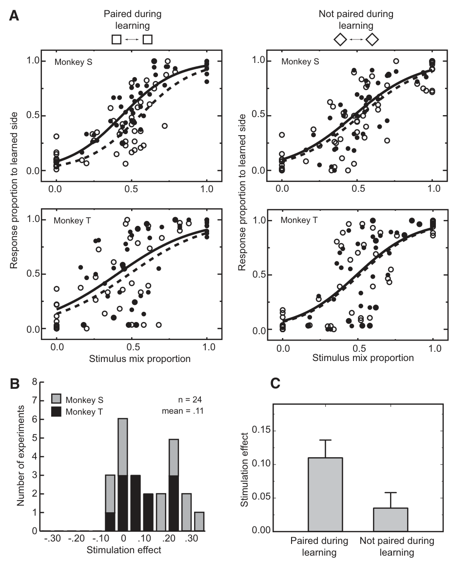
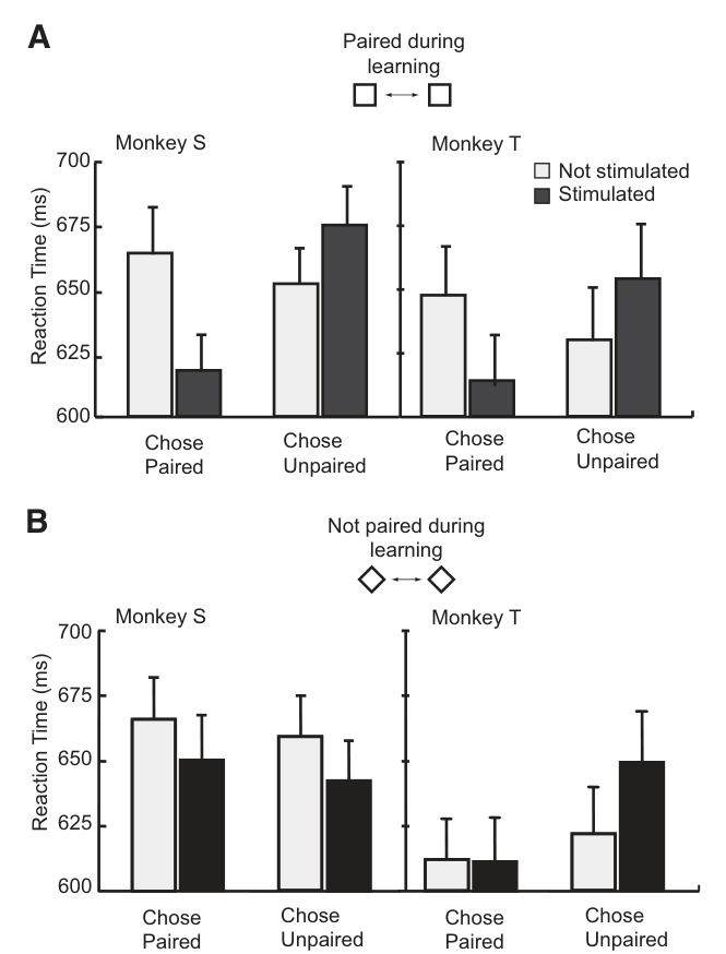
图 8 · 反应时证据:电流影响的是决策时间
原文图注:FIG. 8. Effects of IT microstimulation on reaction times. A: pooled reaction times for ambiguous trials for the response to the stimuli mixture from 1 of which had been previously been associated with microstimulation show that microstimulation affected choice times. Choice reaction times were speeded for stimulated trials in which the monkeys chose the predicted (microstimulation associated) stimulus and were slowed by microstimulation on trials in which the animals chose the unpredicted stimulus (choice × stimulation interaction, monkey S: P < 0.001, monkey T: P < 0.01). Error bars denote 95% confidence intervals. B: pooled reaction times for ambiguous trials in response to the mixtures containing images neither of which had been previously been associated with microstimulation. These data do not show the systematic bias observed for the associated mixtures (choice × stimulation interaction, monkey S: P = 0.2, monkey T: P = 0.1).
解读:纵轴为从视觉出现到按键的反应时间,横轴分"选配对侧"与"选未配对侧"两种选择,条纹区分带电与不带电试次。A 中带电试次在选"预测"侧时变快、在选"非预测"侧时变慢,选择×刺激交互在两猴均显著——电流不仅改变选哪边,还改变到达决策所需的时间,方向与人自主决策中的"证据累积"逻辑一致。B 是未配对混合的对应分析,交互不显著,呼应图 7 的特异性结论。
讨论
作者把本研究与既有微刺激文献对齐:MT、S1、V1 等处的微刺激研究(Salzman et al. 1992; Romo et al. 2000; Tehovnik et al. 2002 等)都假定刺激命中了预先存在的、刺激物调谐过的功能组装;本文没有按选择性挑位点、也没按位点选刺激,而是证明 IT 内存在可被"戳"中的分布式组装池,其与视觉诱发活动的组合足以绑定新联结。与 Doty 的经典皮层条件反射形成对照:那些研究用大电流表面电极、经广泛配对条件化后刺激独自可引出条件反应、而且泛化迅速;本文学习限于单次会话的特定图像,无"学会学习",直接刺激不引发反应,两者任务与刺激方法差异都很大。与 Murphey & Maunsell(2007)的刺激检测训练不同,本文没有给猴子显式的刺激检测训练,而 Afraz 等(2006)在脸区微刺激以约 11% 幅度偏置脸/非脸分类的效果幅度与本文几乎相同——本文位点并非脸部选择区,这提示按非脸性质拓扑聚集的细胞群(Fujita et al. 1992; Tsao et al. 2006)可能同样有效率。作者还讨论一种可能性:学习是在没有显式知觉的情况下发生的(Mishkin 1982; Rosenthal & Behrmann 2006 的病人支持这种分离)。承认的局限说得很明白:结果证明"IT 的差异活动足以建立新联结"并不等于"学习发生在 IT",只能说明刺激与 IT 内的视觉信号发生交互;候选底物包括额-颞交互、颞-缘系统与颞-纹状环路,或 IT 局部回路内类似 Murayama 等(1997)报告的高频刺激引发的突触可塑性——但本文对任何位点都没有长期的细胞反应改变的直接证据。作者最后展望光遗传等新型工具可以让这种"人工活动 - 行为学习"的操纵更特异、更精密度。
一句话总结
这篇的漂亮之处在于用"信息量梯度"把替代解释一个个剥掉:不是刺激-运动直接绑定(纯刺激试次失败),不是检测刺激(相对时序也能学),不是任何皮层电流都行(听觉区失败),也不是泛发的运动效应(偏置带图形特异性)。在我读来,它把 IT 从"学习的关联观察对象"升级成"可人为注入学习信号的处理器"——但也因为如此,单会话内学习快、无跨会话优化这一点让我怀疑真正的联结至少部分写在下游,文中自己也承认了这一点。
审校与证据追溯 (Verification & Evidence)
图表审计结果
- Fig1: 提取质量
good,对齐度full,识别面板[A, B] - Fig2: 提取质量
good,对齐度full,识别面板[A] - Fig3: 提取质量
good,对齐度full,识别面板[A, B] - Fig4: 提取质量
good,对齐度full,识别面板[A, B] - Fig5: 提取质量
good,对齐度full,识别面板[A] - Fig6: 提取质量
good,对齐度full,识别面板[A] - Fig7: 提取质量
good,对齐度full,识别面板[A, B, E, F] - Fig8: 提取质量
good,对齐度full,识别面板[A, B]
关键事实与局限性声明
- 审校纠偏: {'classification': 'OVERCLAIM', 'md_section': '开头定位', 'current_text': '把相关证据……补成了一条因果链。', 'problem': '微刺激是因果操纵,确实支持刺激诱发IT活动对行为学习的充分性;但它不证明正常学习依赖同一活动模式,也不定位可塑性发生在IT。', 'recommended_fix': '改为“提供了关于人工诱发IT活动可支持学习的因果干预证据,但不确定正常学习的可塑性位置”。'} -> 评注:
- 审校纠偏: {'classification': 'OVERCLAIM', 'md_section': '一句话总结', 'current_text': '不是检测刺激(相对时序也能学)。', 'problem': '相对时序结果只排除了“仅检测刺激是否存在”这一简单策略;猴仍可能检测刺激及其时间关系。', 'recommended_fix': '改为“不能仅由刺激存在/缺失检测解释,因为相对时序本身也可成为线索”。'} -> 评注:
- 审校纠偏: {'classification': 'OVERCLAIM', 'md_section': '一句话总结', 'current_text': '不是任何皮层电流都行(听觉区失败)。', 'problem': '只在1只猴中比较了IT与一个邻近听觉反应区,不能推广到所有非IT脑区或所有皮层刺激。', 'recommended_fix': '改为“效应未在所测试的邻近听觉反应区复现,提示一定脑区特异性”。'} -> 评注:
- 审校纠偏: {'classification': 'OVERCLAIM', 'md_section': '一句话总结', 'current_text': '也不是泛发的运动效应(偏置带图形特异性)。', 'problem': '未配对混合仍有3.5%的平均转移,猴S的效应显著;作者明确指出尚需操纵视觉相似性才能区分知觉转移与运动转移。', 'recommended_fix': '改为“图形特异性明显限制了纯粹、完全泛化的运动偏置解释,但没有彻底排除较小的反应侧偏置”。'} -> 评注:
- 审校纠偏: {'classification': 'INTERPRETATION', 'md_section': '一句话总结', 'current_text': '真正的联结至少部分写在下游。', 'problem': '该句已用“让我怀疑”标记为个人推测,因此不属于事实错误;但数据同样允许IT局部回路、额颞、颞缘或颞纹状体环路等多种可塑性位置。', 'recommended_fix': '保留推测标签,并补充“本文无法区分IT局部与下游可塑性”。'} -> 评注:
- 补充要点: : (第 10 页)
- 补充要点: : (第 5 页)
- 补充要点: : (第 10 页)
- 补充要点: : (第 13 页)