IT Literature Intelligence 终审版本 (VERIFIED) 论文编号:
185| 原始基线:V0_ZCODE_BASELINE| 语义审核:needs_revision| 图表审核:pass
Correlated activity supports efficient cortical processing
Hung · Frontiers in Computational Neuroscience · 2014 · Zotero itemID=1704
这篇文章挑战了计算神经科学里一个根深蒂固的直觉——"稀疏、去相关的编码才高效"。作者用覆盖猕猴下颞叶皮层(inferior temporal cortex, IT)约两个皮层柱的 64 位点高密度电极阵,证明少数"合唱者"(choristers,调谐相关且静息时同步放电的神经元)携带比"独唱者"(soloists)更可泛化的物体信息,它们集中在非颗粒层的输出层,而"相关强度"与"调谐锐度"意义上的稀疏性(sparseness)基本无关;更进一步,猴 IT 里由相关结构定义的特征能预测人类视觉搜索的效率。反直觉但证据链完整,值得任何关心群体编码的人细读。
研究背景
视觉识别的核心难题是泛化:表征既要对特定物体敏感,又要对光照、姿态等变化保持不变性(invariance)。主流理论把希望寄托在"高效编码"(efficient coding)上,其中的关键概念是稀疏性——主流看法是,稀疏通过最小化冗余、相关与噪声来提升效率(Gawne 与 Richmond 1993、Vinje 与 Gallant 2000、Ecker 等 2010 等一脉)。但这个框架有个被忽视的漏洞:由于以往电极采样密度不足,多数研究实际测的是"调谐锐度"(单个神经元对刺激集的选择性),却默认它等同于"群体稀疏性"(population sparseness,即同时响应的神经元比例);"相关强度"与"稀疏性"在多样化的 IT 神经样本里究竟什么关系,其实未经检验。另一条线索来自作者团队此前的工作(Lin 等 2014):IT 中少数调谐相关、连自发放电都同步的神经元(choristers,仅约 6%)承载的类内泛化信息,居然抵得上整个阵列的群体,4–5 个合唱者就能达到全阵列的编码能力。
据此作者提出了一个"毛根模型"(pipe cleaner model):绝大多数弱相关的 soloist 像毛根的鬃毛,是 IT 的输入端异质张量;少数强相关的 chorister 像中轴,是 IT 输出的基底,编码支持泛化的不变表征。这个模型给出两个可检验的预测:chorister/soloist 应有层面特异性(输出层 vs 输入层);且这种相关结构应与复杂形状知觉的行为效率挂钩。当时关于相关性的争论(V1 噪声相关到底大不大、是否层面依赖)各执一词,而把局部相关结构、皮层层面与行为三者串起来的实验证据几乎空白——这正是本文要填的缺口。
研究思路
文章的逻辑是"先澄清概念,再找解剖落点,最后接通行为"。第一步,作者意识到必须先回应两个针对其前作(Lin 等 2014)的质疑:chorister 编码更好会不会只是因为它们调谐更宽(对刺激变化更耐受)、或者只是视觉驱动更强、甚至是同一神经元被多个触点重复检出?为此他们直接检验"相关强度 vs 调谐锐度"的关系,并在视觉驱动匹配的条件下重做对比。第二步,层面特异性分析:若模型为真,chorister 应富集在输出层(颗粒层上下的 supragranular/infragranular 层),soloist 应偏向输入层(第 4 层等),这样输入与不变流形(manifold)近正交的安排才说得通。第三步,构造"神经定义特征"(neurally defined features,即由 IT 阵列 PCA 得分极端的刺激集合),拿它们做成人类视觉搜索任务——用"同一柱的相反极性"(opposite)、"同阵列不同主成分"(related)与"不同阵列"(unrelated)三种条件,把 IT 的柱间对比编码与知觉效率直接绑在一起。整个设计刻意避开空间注意与早期视觉因素的混淆:短暂呈现加掩蔽、位置随机化、SHINE 工具箱均衡亮度对比等低级属性。
方法
神经生理部分使用台湾猕猴(Macaca cyclopis)4 只、5 次阵列插入。电极阵为 64 位点(8 柄×8 触点,0.2 mm 间距,覆盖 1.4×1.4 mm),横跨全部皮层深度与约 2–4 个相邻皮层柱,插入外侧 IT(A16)。记录在轻度神经安定麻醉下进行(芬太尼 0.9 µg/kg/hr、70%/30% N₂O/O₂、氟哌利多、0.3–0.5% 异氟烷,加肌松剂),作者论证此浓度远低于会影响神经元动力学的报告值,且麻醉排除了任务相关的自上而下信号与眼动的干扰。刺激为 240 个灰度渲染物体(刺激集 1)与 113 张照片物体(刺激集 2),以快速序列视觉呈现(rapid serial visual presentation, RSVP)播出(94 ms 开/106 ms 关,5 Hz),伪随机顺序重复 10 次,分析取刺激后 100–200 ms 尖峰计数;数据集为 250 个多单元"位点"(site,同一触点分离单元的合并)与来自 359 个神经元的 6462 个位点对。
分析上,每个位点的调谐函数为跨刺激 z 归一化的平均反应;以每位点与同阵其他位点的平均两两调谐相关(average correlation strength)排序,前 30% 分位为 chorister(5 个阵列的平均相关强度为 0.15±0.04),行为对比中的 soloist 取 45–65% 分位(层面分析则取底部 30%,平均 0.02±0.03)。稀疏性按 Vinje 与 Gallant(2000)、Zoccolan 等(2007)的修正指数计算。类内泛化能力用线性支持向量机(support vector machine)评估:8 类各学一个 one-vs-all 超平面,对未见过的物体做分类(随机水平 12.5%)。低维结构用主成分分析(principal component analysis, PCA)从 240×64 的 z 归一化反应矩阵提取,PC1 大致对应全阵列的共激活/共抑制,PC2 对应相邻两柱的差分激活;噪声相关(noise correlation, Rsc)衡量成对位点的逐试次共变。人类实验为 6 名观察者(3 男 3 女,除第二作者外不知实验目的):四象限中 1 个目标加 3 个干扰物叠在适应背景上,背景先行呈现 0–8 s,目标组呈现 34–136 ms 后打掩蔽,按键报告目标所在象限(随机水平 25%),每条件 48 试次,目标/干扰/背景分属互不相交的神经定义特征集合。
主要结果
-
相关强度与稀疏性基本无关:250 个位点上二者总体相关仅 r=−0.09(p=0.04,图 2A),且在 5 个阵列内部各自不显著;而两项测量各自在两个刺激集间高度稳定(r=0.72 与 0.70,p<10⁻³⁷ 与 p<10⁻³⁹),说明弱相关不是噪声所致。这直接否定了"chorister 编码好是因为调谐宽"的平凡解释,也说明以往把调谐锐度当群体稀疏性的做法站不住脚。
-
合唱者的编码优势与更强的噪声相关,且在视觉驱动匹配后依然成立:chorister 的类内泛化解码表现优于 soloist(图 2B),即便把两者匹配到对偏好刺激约 12 spikes/s 的基线扣除反应后仍如此;chorister 对的噪声相关 Rsc=0.13,soloist 对仅 0.04(p<10⁻²²,图 2C),只取视觉驱动相近(10–30 spikes/s)且水平距离≥0.6 mm 的位点对时为 0.16 对 0.06(p<10⁻¹³)。
-
相关神经元集中在输出层:64 个 chorister 中仅 5 个位于 1.0–1.2 mm 深度(第 4 层附近),其余都在颗粒层上下(图 3A);最不相关的 soloist 反而在 0.2 mm 与 1.2 mm 深度(第 1、4 层)更常见(图 3B)。颗粒层中 chorister 比例显著更低(Fisher 精确检验 p=0.0007 与 p=0.0003)。与此形成对照,稀疏性本身没有层面特异性(图 3C,D,均不显著)。
-
低维相关结构同样集中于输出层:阵列内前两个主成分只解释约 25% 的反应方差;单个位点被前两个 PC 解释的方差比例(%EV)在 0.2 mm 与 1.2 mm 深度显著更低(许多位点 <5%EV),而在颗粒层上下的位点可高达 77%(图 4D,E)。将 PC 得分的刺激标签打乱后 %EV 平均为 −23%,说明这些位点确实是被视觉驱动且选择性的;唯有第 4 层的平均反应低于基线(−0.5 spikes/s),符合前馈/局部抑制造成的压抑。作者解读为:IT 的输入(前馈与反馈)与相关流形近乎正交,而相关结构由局部回路塑造。
-
改为“猴IT神经定义特征预测短暂掩蔽条件下的人类目标定位正确率,作者将该指标称为视觉搜索效率”。:PC2− 极端的刺激多为带突起的物体,PC2+ 极端多为带内部特征的物体(定性标签,不进入特征定义,图 5)。行为上,34 ms 呈现时目标与干扰/背景属"相反"特征(差分驱动相邻柱)的准确率高于"相关"特征:单被试 p=0.038(Cochran-Mantel-Haenszel 检验),6 名被试在 2 s 适应下 p=0.03(Wilcoxon 符号秩检验,图 7B);且该效应只在最短 SOA(34 ms)出现,适应 8 s 时则所有 SOA 上都成立。"相关"(0 mm 皮层间距)与"不相关"(>3 mm)条件之间无显著差异,"相反"优于"不相关"也仅在 4/6 被试中出现且未达显著——指向短程侧向抑制而非距离效应。
图注解读
图 1 · 实验设计与毛根模型
原文图注:FIGURE 1 | Experimental design and "pipe cleaner" model. (A) We inserted a dense multi-depth array (64 sites across ∼2 cortical columns) in macaque lateral IT (A16) and recorded spiking responses under light neurolept anesthesia. Stimuli were presented via rapid serial visual presentation, for 94 ms ON and 106 ms OFF (5 Hz), in pseudorandom order for 10 repetitions. Spike count from 100 to 200 ms post stimulus onset was averaged across repetitions. (B) A "pipe cleaner" model linking local correlational structure in neighboring columns to invariant representation. Most neurons are weakly correlated "soloists" (the bristles), tied to an underlying structure of correlated neurons ("choristers", the spine). Sampling a few points along the spine (a few choristers) is sufficient to reconstruct the overall structure. The model predicts that generalizable object information is carried by the choristers, and that the heterogeneity of the soloists may help to fine-tune the choristers to support generalization.
(A) 交代记录与刺激呈现的所有硬参数:64 位点阵列、轻度麻醉、RSVP 的 5 Hz 节律、100–200 ms 计数窗。(B) 是全文的概念图:鬃毛(soloist)是输入端的异质张量,中轴(chorister)是输出的不变表征,沿中轴取几个采样点即可重建整体结构——这解释了为什么 4–5 个 chorister 就有全阵列的编码能力,也预告了层面特异性的预测。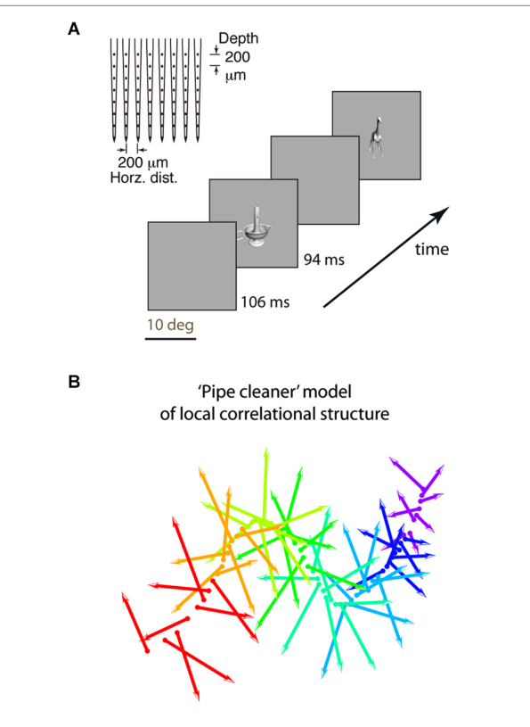
图 2 · 相关结构、稀疏性与泛化解码
原文图注:FIGURE 2 | Local correlational structure, sparseness, and generalization performance. (A) Sparseness (tuning width) and average correlation strength were only weakly related across 250 sites in anesthetized IT (r = −0.09, p = 0.04). Sparseness and average correlation strength were each highly consistent across two stimulus sets (r = 0.72 and 0.70, p < 10−37 and p < 10−39 resp.). Choristers (brown) are the 30%ile of sites with the highest average correlation strength per array, and soloists (black) are the remaining sites. (B) Visual responsiveness vs. within-category generalization performance for choristers (top 30%ile, brown) vs. soloists (45–65%ile, red), for 2 sites per array, with at least 600 µm horizontal distance between sites. Visual responsiveness was calculated as the evoked (baseline-subtracted) response to each site's preferred object, shown as the median across 10 sites (2 sites per array, 5 array insertions across 4 monkeys). Chance is 12.5% for 8 categories, and ceiling performance is based on all sites. (C) Noise correlation (Rsc) of choristers vs. soloists ... (D) Same analysis based on sparseness (tuning sharpness). Average sparseness of broadly tuned and sharply tuned (sparse) sites were 0.12 ± 0.08 and 0.69 ± 0.25, resp.
读法:(A) 是散点图,横轴稀疏性、纵轴平均相关强度,肉眼可见几乎无趋势(r=−0.09);(B) 中棕点(chorister)的泛化解码表现系统性高于红点(soloist),且这是在视觉驱动匹配与 ≥600 µm 水平距离约束下取得的,排除"同一神经元重复检出"与"驱动差异"两个平凡解释;(C) 的 Rsc 对比(0.13 对 0.04)说明调谐相关伴随更强的逐试次共变;(D) 显示按稀疏性分组做同样分析得不到编码差异。这张图支撑结果第 1、2 条,是"概念解绑"的核心证据。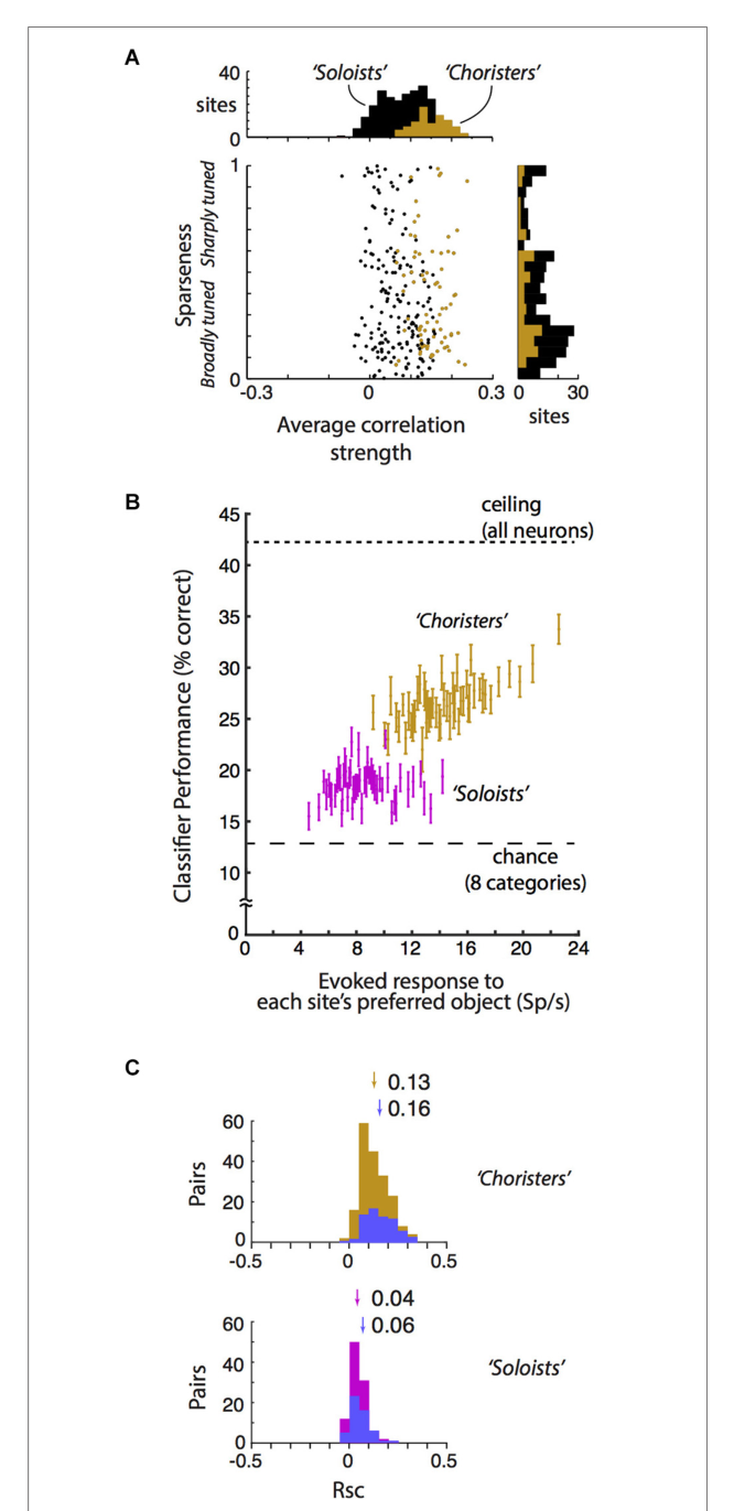
图 3 · 皮层深度与相关强度/稀疏性
原文图注:FIGURE 3 | Cortical depth vs. correlation strength and sparseness. (A,B) We sorted sites by their average strength of tuning correlation with other sites in the same array, then grouped the top ∼30% of sites per array as "choristers" and the bottom ∼30% as "soloists". Choristers are rarer in layer 4 (1.0–1.2 mm depth), whereas soloists are more common at 0.2 and 1.2 mm depth. The number of sites selected per group was higher for arrays 1–3 (16 choristers and 16 soloists per array) than for arrays 4 and 5 (8 choristers/soloists per array), because arrays 4 and 5 had fewer active channels. Average correlation strengths of choristers and soloists were 0.15 ± 0.04 and 0.02 ± 0.03, resp. (C,D) Same analysis based on sparseness (tuning sharpness). Average sparseness of broadly tuned and sharply tuned (sparse) sites were 0.12 ± 0.08 and 0.69 ± 0.25, resp.
按皮层深度(0.2 mm 起、每 0.2 mm 一档,至 1.2 mm 以上)统计 chorister 与 soloist 的出现比例:(A)(B) 显示 chorister 在第 4 层附近(1.0–1.2 mm)几乎绝迹,soloist 在 0.2 与 1.2 mm 处富集;(C)(D) 做同样的深度分析但按调谐锐度分组,结果无层面差异。一有一无的对比非常干净:层面特异性属于相关结构而非稀疏性,支撑结果第 3 条。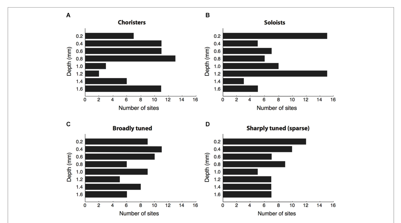
图 4 · 皮层深度与低维相关结构
原文图注:FIGURE 4 | Cortical depth vs. low-dimensional correlational structure. (A) Percent of response variance explained by PCs 1–5, based on z-normalized responses. Chance and 5–95%ile distributions are indicated by open circles and red bars, based on shuffling of response IDs across trials. (B,C) Explained variance for Arrays 2 and 3, from two separate array insertions (separate recording sessions) in monkey 2. (D) Cortical depth vs. percent explained variance of PCs 1 and 2 across 5 arrays. (E) Comparison of distributions in (D) among different depths. p < 0.05, p < 0.01, **p < 0.001, •p = n.s.
(A) 给出每个 PC 解释方差的比例与打乱标签后的随机水平对照;(B)(C) 是两个示例阵列的逐位点 %EV 空间图,可见输出层的位点被前两个 PC 解释得更好;(D)(E) 汇总 5 个阵列,按深度比较 %EV 分布,0.2 mm 与 1.2 mm 深度显著更低。这张图把"层面特异性"从分组统计(图 3)推进到低维流形层面,支撑结果第 4 条,也是"输入近正交于流形"这一模型推论的直接证据。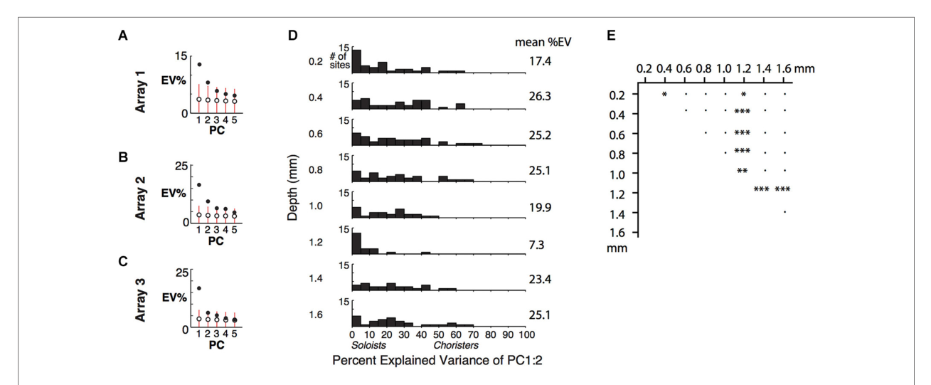
图 5 · 神经定义特征长什么样
原文图注:FIGURE 5 | Neurally defined features. (A) Neurally defined features based on Array 1's PC1 and PC2 scores. Each red and blue 8 × 8 matrix shows baseline-subtracted response to one stimulus across the 64 sites, spanning all depths and neighboring IT columns. PC1+ stimuli activated most sites. PC2+ and PC2− stimuli differentially activated sites on the right and left sides of the array. Numbers indicate stimulus IDs. Black dots in stimulus 19's matrix indicate inactive sites. Red lines indicate 5–95%ile, and filled circles indicate stimuli with significant PC2. "Protrusions" and "Internal Features" are labels to help see the pattern of PC2− and PC2+ stimuli, but the labels are not part of the feature definition. (B) Features from 3 array insertions (3 recording sessions) in two monkeys and two stimulus sets. Only the stimuli with the most extreme scores are shown, out of 240 object stimuli for set 1 (grayscale rendered 3D objects) and 113 stimuli for set 2 (color, grayscale, and silhouette photographs).
(A) 中每个 8×8 色块矩阵是一个刺激在 64 个位点上的基线扣除反应:PC1+ 刺激激活大部分位点,PC2+/PC2− 刺激则分别偏向阵列右/左侧(即相邻两柱之一)。注意"突起/内部特征"只是帮助读者看出规律的语义标签,特征定义完全由 PCA 得分极端性决定。(B) 展示来自两只猴三次插入、两个刺激集的极端刺激样本。这张图是从神经测量走向行为刺激的桥梁,支撑结果第 5 条的前置设定。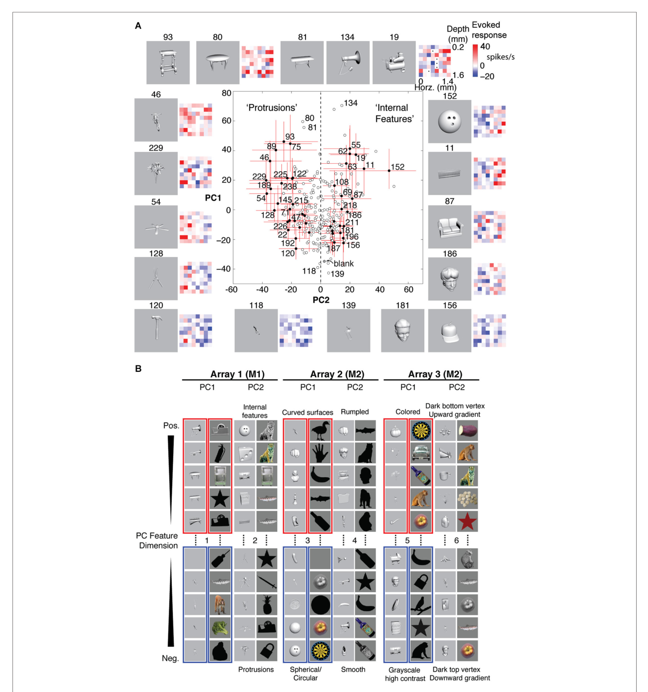
图 6 · 基于神经定义特征的视觉搜索任务
原文图注:FIGURE 6 | Visual search task based on neurally defined features. (A) "Related", "Opposite", and "Unrelated" conditions are tied to the differential activation of overlapping, neighboring, and distant IT columns by neurally defined features. In each condition, the target objects belong to one feature (e.g., Array 2 PC2+) and the distractor and background objects are disjoint sets belonging to the other feature (e.g., Array 2 PC2−). "Related" features are from different PCs of the same array. "Opposite" features are from opposite signs of the same PC of the same array. "Unrelated" features are from different arrays. (B) Time course of each trial. Following Fixation screen and Adapting Background (0–8 s), Target and Distractors appeared for 34–136 ms, followed by a Mask with tile-scrambled background images. After disappearance of the fixation point, subjects reported via keypress the target quadrant. (C) Each trial consisted of one target and 3 distractors at four possible locations. Objects and target locations were balanced across all conditions. (D) Example stimulus from "opposite" condition, with target in quadrant 4.
(A) 定义三种条件的皮层几何含义:opposite=同一 PC 的相反极性(相邻柱差分)、related=同阵列不同 PC(同一柱的不同尺度)、unrelated=不同阵列(相距 >3 mm 的柱);(B) 给出试次时序(注视→适应背景 0–8 s→目标组 34–136 ms→掩蔽→按键报告象限);(D) 是 opposite 条件的实际画面示例。三种条件把"皮层邻近性"变成了实验自变量,支撑结果第 5 条的设计逻辑。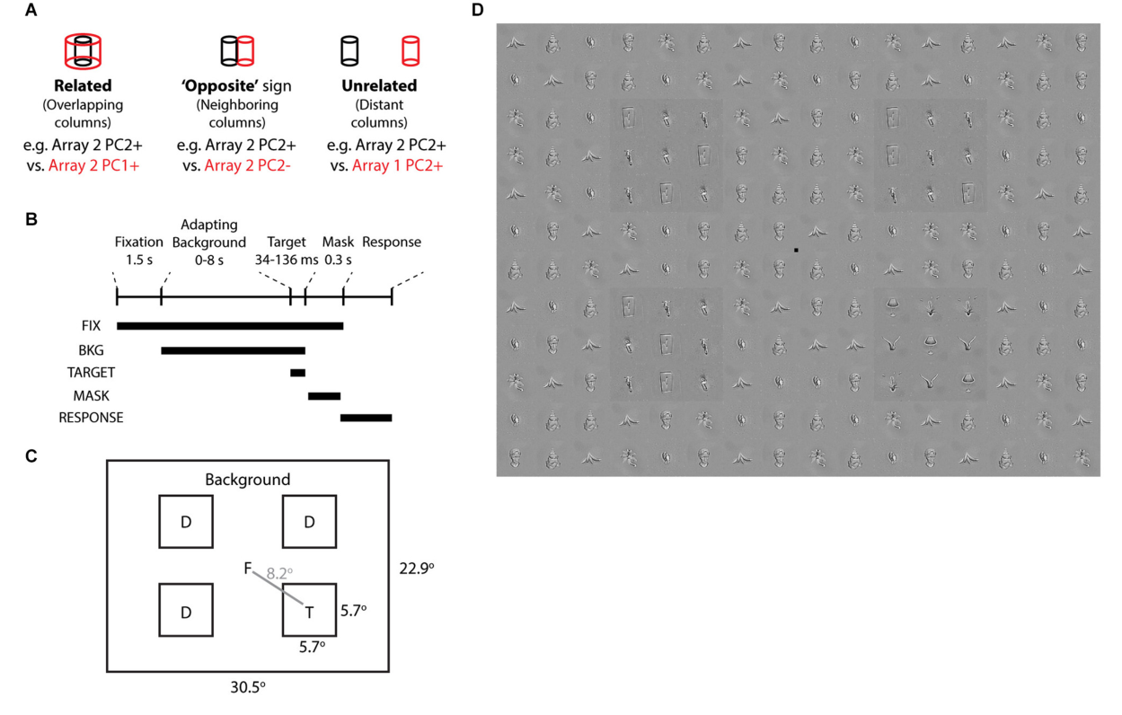
图 7 · 神经定义特征的视觉搜索表现
原文图注:FIGURE 7 | Visual search performance for neurally defined features. (A) Performance of one subject for target whose neurally defined feature is "opposite" (blue) or "related" (red) to that of the distractors and background, across different adaptations and different stimulus onset asynchrony (SOA) between stimulus and mask. Accuracy is higher for "opposite" at 34 ms SOA, and the difference between "opposite" and "related" is more consistent at longer adaptation. Error bars show 95% CI, based on 48 trials per condition. (B) Performance across 6 subjects at 2 s adaptation and 34 ms SOA for "opposite" (blue), "related" (red), and "unrelated" (green) conditions. Black line indicates average performance across subjects. The difference between "opposite" and "related" is significant at p = 0.03, based on Wilcoxon signed ranks test. (C) Average performance across 6 subjects at 34, 68, and 136 ms SOA, 2 s adaptation.
(A) 单被试的准确率随适应时长与 SOA 变化,蓝色(opposite)在 34 ms SOA 稳定高于红色(related);(B) 6 名被试在 2 s 适应、34 ms SOA 下的个人成绩与均值,opposite 对 related 的差达显著(p=0.03);(C) 显示把 SOA 拉长到 68、136 ms 后组间差异消失。正是"只在最短 SOA 出现"这一点支持了效应来自前馈加工与短程侧向相互作用,而非反馈或长程交互,支撑结果第 5 条。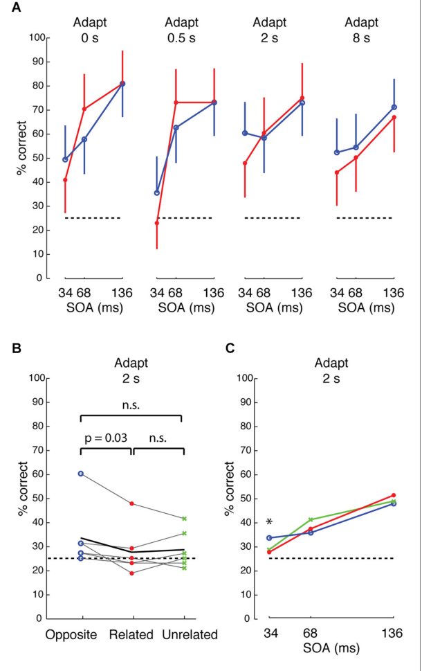
讨论
作者的结论是三连击:相关强度与稀疏性应作为两个独立因素对待(相关强度才是群体冗余的更好度量);相关活动主要位于输出层(方向与"稀疏提升效率"的预期相反);猴 IT 的相关活动预测人类视觉搜索效率。机制上,作者推测第 1、4 层的前馈与反馈输入本身已去相关或被抑制主动去相关,而输出层的局部回路与水平纤维产生相关结构;若如此,输入的异质性(群体稀疏)与输出的冗余/平滑(调谐重叠)的组合,可能正是二元放电神经元在高维特征空间中解决"位分辨率"不足的方案。与模型的对话相当直接:卷积网络在 ImageNet 上虽胜过尖峰网络、甚至超过随机采样的 IT 神经元,但 Yamins 等 2014 的最优模型对 IT 单个位点的拟合可低至 20%EV(均值 48.5%EV),作者认为差距部分来自随机池里 soloist 占多数,主张把基准换成 IT chorister;行为端则与特征整合理论(feature integration theory)对话——快速搜索不再只属于早期视觉区的低级特征,特定类型的复杂特征也能被前注意并行搜索,这与 Duncan 与 Humphreys 的"搜索皆并行、取决于表征相似性"模型相合。作者亦坦承局限:神经数据是麻醉下对既有数据集(Lin 等 2014)的再分析,皮层深度靠插入过程目测追踪而非组织学确认(偏差估计 <8°);效应量在行为端不大且仅在最短 SOA 显著。他们还联想到自闭症中物体区相关活动与兴奋/抑制平衡异常可能对应知觉异常,并呼吁用 64 神经元/mm³ 量级的高密度阵列才能测量群体稀疏性。
一句话总结
在我看来,这篇文章的锐利之处在于它戳破了一个概念偷换:大家嘴上说"稀疏编码高效",手上量的却是调谐锐度,而真正与冗余相关的那件事——群体相关结构——被高密度阵列翻出来后,居然指向输出层更相关、且相关者编码更好。当然要留个心眼:数据来自轻度麻醉下的再分析,chorister/soloist 只是人为切分的连续谱两端,行为效应也偏小;但"输入异质、输出冗余"这个架构图像一句值得带进任何群体编码讨论的话。
审校与证据追溯 (Verification & Evidence)
图表审计结果
- Fig1: 提取质量
good,对齐度full,识别面板[A, B] - Fig2: 提取质量
good,对齐度full,识别面板[A] - Fig3: 提取质量
good,对齐度full,识别面板[A, B] - Fig4: 提取质量
good,对齐度full,识别面板[A, B, C] - Fig5: 提取质量
good,对齐度full,识别面板[] - Fig6: 提取质量
good,对齐度full,识别面板[A, B] - Fig7: 提取质量
good,对齐度full,识别面板[A, B]
关键事实与局限性声明
- 审校纠偏: 证明少数chorister携带更可泛化的信息 -> 评注:
- 审校纠偏: 输入近正交于流形的直接证据 -> 评注:
- 审校纠偏: 效应来自前馈加工与短程侧向抑制,而非反馈或长程交互 -> 评注:
- 补充要点: : (第 3 页)
- 补充要点: : (第 3 页)
- 补充要点: : (第 11 页)
- 补充要点: : (第 8 页)
- 补充要点: : (第 12 页)
- 补充要点: : (第 10 页)