IT Literature Intelligence 终审版本 (VERIFIED) 论文编号: 147 | 原始基线: V0_ZCODE_BASELINE | 语义审核: fail | 图表审核: pass

Organization of Local Horizontal Functional Interactions Between Neurons in the Inferior Temporal Cortex

Tamura · Journal of Neurophysiology · 2014 · Zotero itemID=1458

这篇实验论文用八轴四分簇电极阵列在猕猴下颞皮层（inferior temporal cortex，IT）同时记录最大相距 1.4 mm 的神经元对，用毫秒尺度的互相关分析描绘了"水平方向功能连接的组织规则"：连接随皮层距离衰减，且偏好越相似连接越强；更妙的是，作者发现"偏好相似性对连接强度的约束"在远距离神经元对之间反而比相邻对更突出。这篇文章值得读，因为它把 IT 皮层功能结构的问题从"有没有连接"推进到"不同距离尺度的连接承担不同功能"——这直接关系到物体表征如何在局部组合与长程整合之间分工。

研究背景

皮层回路结构的知识是理解信息加工机制的前提。从形态学看，皮层锥体神经元的基树突通常横跨约 0.4 mm，因此相距小于 0.4 mm 的相邻神经元树突野重叠、很可能共享输入；在初级视皮层（V1），相邻神经元之间确实比分开的神经元更常有功能连接，而且偏好相似（如同方位偏好）的神经元倾向于功能连接——V1 的"接线图"已画得相当清楚。IT 皮层则不同：它处于腹侧通路末端、对物体识别至关重要，其锥体神经元的树突野更大、水平轴突分布更广；同时 IT 相邻神经元共享刺激偏好的程度远弱于 V1（有研究认为 IT 缺乏像 V1 那样清晰的柱状功能组织）。形态与功能组织的双重差异都提示，IT 的回路组织原则可能与 V1 不同，但当时对纹外皮层回路组织的了解非常有限。

在方法学层面还有一个空白：功能交互历来靠 spike-to-spike 相关在毫秒尺度上评估，而既往对清醒/麻醉猴 IT 的功能连接研究只覆盖了相距不足 0.5 mm 的神经元对，"横向分离的 IT 神经元之间是否存在毫秒级功能交互、其组织规则与相邻对有何不同"完全没有数据。本文正是要同时填补这两层空白——距离维度（0 到 1.4 mm）与偏好相似性维度——的交叉。

研究思路

作者的策略可以概括为"一箭双雕的记录平台加三重关联分析"。用一排八个四分簇电极（tetrode）一次穿刺，把 IT 第 2/3 层内 0–1.4 mm 范围的多个神经元同时抓住：同一轴（0 mm 距离）提供真正的相邻对，跨轴（0.2–1.4 mm）提供不同尺度的横向分离对。对每对神经元并行计算三类指标——刺激偏好相似性（signal correlation）、试次间波动一致性（noise correlation）与毫秒级功能交互（互相关图，cross-correlogram，CCG）——然后在两个维度上考察连接的组织：距离如何影响交互的存在概率与强度，偏好相似性又如何与交互强度挂钩。

真正新颖的是第三步：把两个维度交叉起来，分距离组比较"CCG 峰高与偏好相似性"的相关系数。如果 IT 的水平连接与 V1 一样属于"近邻随意、远距按功能挑选"的模式，那么"距离越远、约束越强"的预测就能被直接检验。作者并不满足于此——所有随距离出现的关系都被用对照分析排查了替代解释（峰分离错误、放电率、样本量、CCG 形状等），这种层层设防的设计保障了"回路组织本身不同"这一最终结论。

方法

被试为两只雄性猕猴（Macaca fuscata 与 Macaca fascicularis，体重 6.0 与 2.9 kg），共 3 个半球 7 次电极穿刺（一只 2 次、另一只 5 次），分别记录 59 与 148 个神经元。记录部位在耳道前方 7.2–15.8 mm、背侧 0.5–11.1 mm，即上颞沟与前中颞沟之间、后中颞沟之前的 IT 皮层（感觉野均大于 10°，多数穿刺位于细胞构筑区 area TE）。实验在麻醉、肌松条件下进行（记录期以潘库溴铵抑制眼动），八轴电极阵列相邻轴间距 0.2 mm、每轴尖端 4 个记录点间距 25 µm，轴平行于皮层表面缓慢插入，推定记录自 IT 第 2/3 层；信号放大 1 万倍、带通 500–3000 Hz、以 50 µs 分辨率数字化。

单细胞分离用四探针协方差向量的层级聚类完成，并以信噪比与 Mahalanobis 距离把关：纳入神经元的中位 SNR 为 22.7 dB；分析仅保留 D²>10.82（约 5% 错分率）的神经元对，其中 90% 的对 D²>21.6（错分率小于 1%）。视觉刺激为一套 100 张图（猴脸 13、人脸 9、其他动物脸 3、手 1、动物身体 3、人体 9、无生命物 3、植物 5、食物 3、二维几何形状 37、纹理图案 13、灰空白 1），多数约 4° 视角，单眼呈现于记录半球对侧眼、置于中央凹 0.5 s，间隔 0.5 s，每 session 重复 30 个 block，每 block 每图出现一次。响应幅度取刺激后 0.5 s（起点后移 80 ms 补偿延迟）、30 试次平均；197/207 个神经元有显著视觉反应。

功能交互用 CCG 评估：1 ms 分辨率、±0.25 s 窗、以两神经元锋电位数的几何平均归一化；用 shift-predicted CCG（试次错位重配）扣除非神经网络性的刺激锁定成分，只有原始 CCG 中扣余后仍显著（二项检验 p<0.0001）的 0 ms 附近峰才算功能交互。偏好相似性以 signal correlation（两神经元对 100 刺激响应谱的 Pearson 相关）度量；试次间波动一致性以 noise correlation（单试次响应 z 评分后的 Pearson 相关）度量。4191 个神经元对（来自 197 个视觉响应神经元）构成分析主体。

主要结果

1. 相邻对的功能交互更强更普遍，但远至 1.4 mm 的对仍有显著交互。4191 对中 17%（732 对）有显著 CCG 峰；显著峰的出现概率随距离骤降：相邻对（0 mm）为 46%，0.2 mm 为 24%，0.4 mm 及更远不超过 11%（图 7C）。峰高同样随距离衰减：相邻对中位峰高 0.0048，0.4 mm 及更远不超过 0.003（图 7D）；即便仅取有显著峰的对，相邻对（0.0073）也高于 1.4 mm 对（0.0044）。

2. IT 神经元携带冗余但偏少的信号相关与噪声相关。全体 4191 对的 signal correlation 中位为 0.07（显著大于 0；19% 的对显著正相关、1% 显著负相关，打乱对照数据的中位为 −0.007）；noise correlation 中位为 0.02（35% 的对显著正、2% 显著负）。两者都随距离下降：signal correlation 从相邻对的 0.24（中位）一路降至 0.4 mm 以外的不足 0.1，noise correlation 从 0.09 降至 0.4 mm 以外的不足 0.025（图 5E、6D），剔除同轴记录对后趋势不变。

3. 功能交互强度与刺激偏好相似性正相关。CCG 峰高与 signal correlation 在全体对上相关（r=0.31, p<0.001）、与 noise correlation 相关更强（r=0.50，符合理论预期，属确证性结果）（图 8）。联合分析显示：偏好高度相似（signal correlation 0.65–0.75）的相邻对中 70% 有显著峰、中位峰高 0.011；试次波动高度一致（noise correlation 0.25–0.35）的相邻对中 100% 有显著峰、中位峰高 0.016（图 9）。

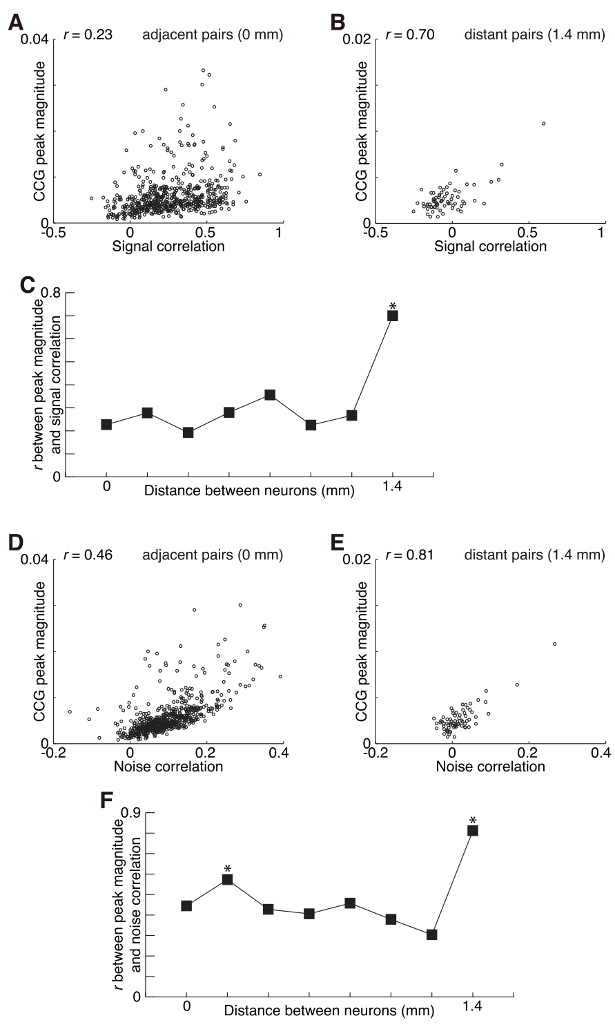
4. 全文最关键的发现：偏好相似性对连接强度的约束随距离增强。CCG 峰高与 signal correlation 之间的相关系数从相邻对的 0.23 升至 1.4 mm 对的 0.70（差异 p<0.001，Fisher 变换检验）；noise correlation 侧从 0.46 升至 0.81。匹配两类对的 signal correlation 范围、剔除同轴对、剔除高放电率影响、限峰高样本量等对照之后，这一梯度的结论依然成立（图 10）。

5. 替代解释被逐一排除。spike 分选错误不能解释距离效应（剔除 0 mm 对后三个相关度量仍与距离负相关）；CCG 形状差异（以峰面积比量化）与峰高–noise correlation 相关强度无关（r=0.13, p=0.76）；相邻对与最远对的锋电位数相当（中位 5050 对 4760，p=0.97）；对数差异贡献甚微（从 565 个相邻对中随机抽 70 对、1000 次的平均相关为 0.54，仍显著小于最远组的 0.81）。作者据此断定差异来源于底层神经回路本身。

图注解读

图 1 · 实验方法总览

原文图注：Fig. 1. Experimental methods. A: recording sites in three hemispheres of two monkeys are marked with circles on the left hemisphere of a cynomolgus monkey. amts, Anterior middle temporal sulcus; pmts, posterior middle temporal sulcus; sts, superior temporal sulcus. B: schematic of the tetrode array (left) and an enlarged image of a shaft tip (right). The array consists of eight shafts (numbers 1–8). The distance between adjacent shafts is 0.2 mm. The length of each shaft is 2 mm. Four recording probes at the tip of each shaft form a tetrode (channels 1–4). The distance between adjacent probes is 25 m. Images are not drawn to scale. C: an example of signals recorded from a tetrode. D: frequency distribution of the signal-to-noise ratio (SNR; dB) of spikes from 207 isolated neurons. E: freq……

这张方法总图给出四样东西：A 为两个猴三个半球上的记录位点（位于 STS 与前中颞沟之间的 IT）；B 为八轴四分簇阵列的示意图与轴尖放大图（轴间距 0.2 mm、探针间距 25 µm、覆盖 1.4 mm）；C 是一路 tetrode 的四通道原始信号示例；D 是 207 个分选神经元的 SNR 分布（中位 22.7 dB）。它支撑方法部分的核心：跨越 1.4 mm 的高质量并行单细胞记录是后文一切距离分析的地基。

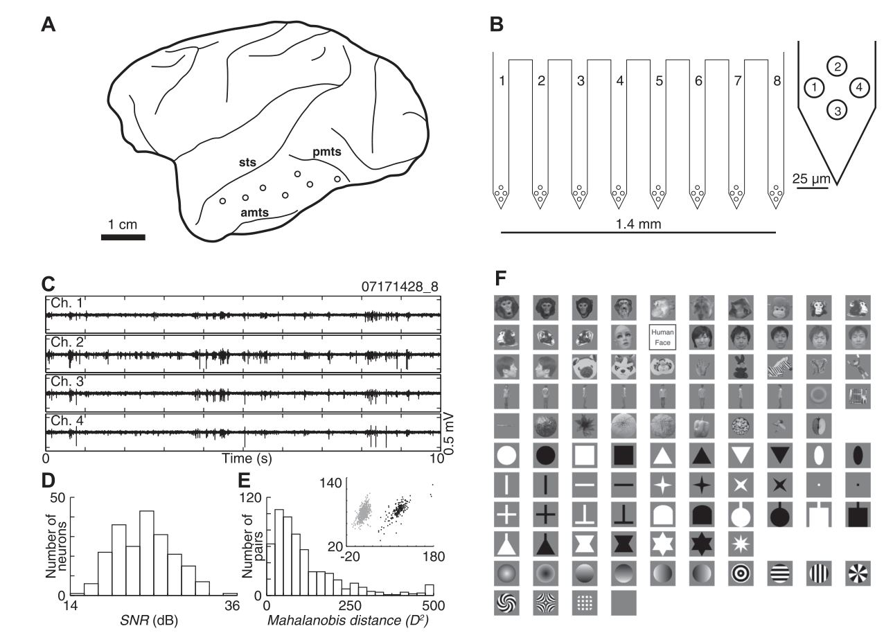
图 2 · 相邻神经元对的响应与三类相关度量

原文图注：Fig. 2. Example of responses and correlation measures of adjacent inferior temporal (IT) neurons recorded from a tetrode (distance, 0 mm). A: the average spike waveforms of cells 1 (left panel) and 2 (right panel) recorded from four probes (channels 1–4) of a tetrode. B: peristimulus time histograms (PSTHs) reflecting the responses of cells 1 (left panel) and 2 (right panel) to the stimulus set. PSTHs are arranged in the same order as the stimulus images in Fig. 1F. Firing rates (spikes/s) are plotted for a 1-s period with a 20-ms bin width. Vertical dotted lines within each PSTH indicate stimulus onset and offset. Each stimulus was presented for 0.5 s. Stars in the PSTHs indicate significant differences between the firing rates during visual stimulation and spontaneous fir……

读法：A 面板显示两细胞在四探针上的平均波形形状不同，说明是两个真正分开的神经元；B 面板按刺激顺序排列两细胞的 PSTH，可见两者都被第 14 号"假人面孔"图强激活；C 面板以每一点对应一个刺激的试次平均响应，给出 signal correlation=0.65；D 面板每点对应单试次 z 评分响应，noise correlation=0.23；E 面板的 CCG 在 0 ms 处有一个显著尖峰（峰高 0.021），而 shift-predicted 对照几乎平坦。此图是全部三个度量的实例教学，支撑结果 3 中"偏好相似的相邻对交互强"。

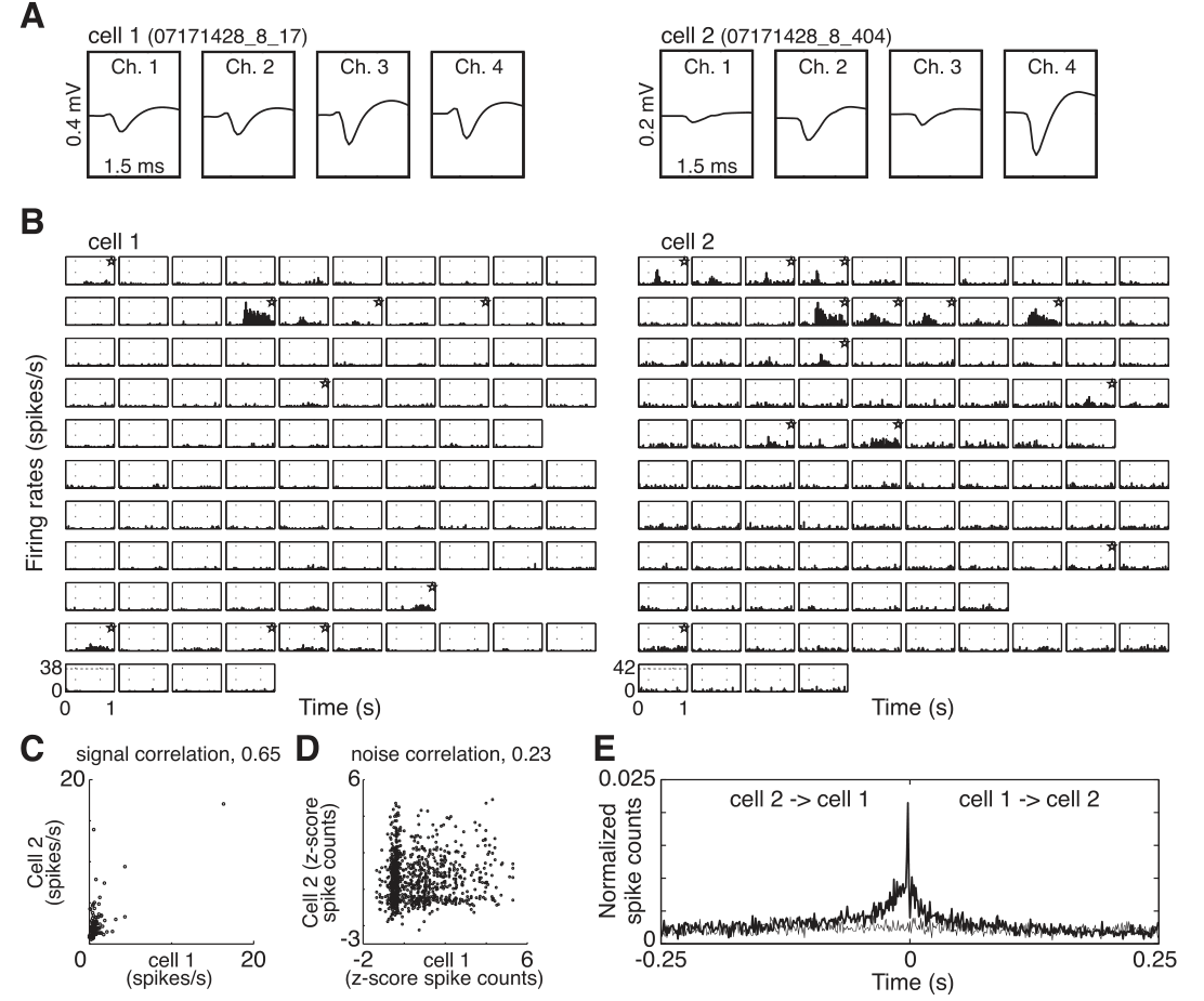
图 3 · 相邻弱关联对与远距离对的 CCG 对照

原文图注：Fig. 3. Two examples of CCGs between neurons in IT cortex. A and B: plots of signal (A) and noise (B) correlation between cells 1 and 2 recorded from a tetrode (distance, 0 mm). C: CCG between cells 1 and 2. Number of spikes: 6,331 for cell 1 and 12,250 for cell 2. D and E: signal (D) and noise (E) correlation between cells 3 and 4 recorded from the first and the eighth shaft of a tetrode array (distance, 1.4 mm). F: CCG for cells 3 and 4. Number of spikes: 5,454 for cell 3 and 12,318 for cell 4. Other aspects of the figure are as described for Fig. 2.

读法：上半（A–C）是另一对相邻神经元：signal correlation 弱（0.10, p=0.31）、noise correlation 低但显著（0.25），CCG 峰较低（0.011）——说明相邻对即便有峰，偏好也未必相似；下半（D–F）是来自第一轴与第八轴、相距 1.4 mm 的对：signal correlation 中等（0.30）、noise correlation 很低但显著（0.07），CCG 仍有小而显著的峰（0.0048）。这两例支撑结果 1 的另一半：远距离对确有真实交互，只是幅度小。也引出全文的核心问题——什么样的远距离对会保留连接。

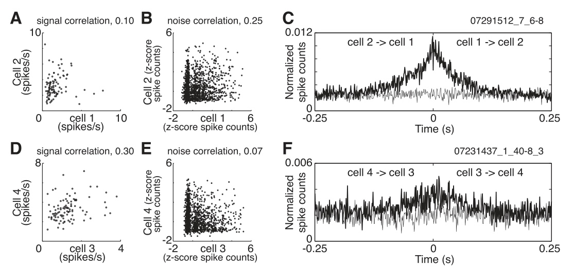
图 4 · IT 神经元的选择性稀疏程度

原文图注：Fig. 4. Sparseness for 197 visually responsive IT neurons. A and B: frequency distribution of sparseness calculated with raw firing rates (A) and that with baseline-subtracted firing rates (B). C: relationship between sparsenesses calculated from raw and baseline-subtracted firing rates.

读法：sparseness 指数衡量神经元响应分布的稀疏性：只对一个刺激强响应为 1，对所有刺激均匀响应为 0。A 用原始放电率算，全群中位数 0.29；B 扣除自发基线后算，中位数升至 0.74；C 显示两者正相关（r=0.47, p<0.001），故后文统一采用原始放电率版。此图为刺激选择性的度量奠定基础，并交代了它与后文相关度量的弱关联（signal correlation 与 sparseness 仅 r=0.07）。

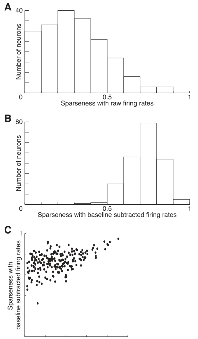
图 5 · 4191 对神经元的 signal correlation

原文图注：Fig. 5. Signal correlation of 4,191 IT neuron pairs within 1.4 mm of each other. A and B: frequency distribution of signal correlation (A) and signal correlation calculated using one set of shuffled data (B). Filled column, significant correlation (P < 0.01, test for independence). Open column, nonsignificant correlation. C: relationship between firing rate and signal correlation. The geometric mean of the maximum firing rate of two neurons in a pair represented the firing rate of the pair. D: relationship between sparseness and signal correlation. The average sparseness calculated from raw firing rates of two neurons in a pair represented the sparseness of the pair. E: relationship between signal correlation and neuron distance. We divided neuron pairs into eight groups according to the distance……

读法：A 是全体对的 signal correlation 分布（实心柱为按独立性检验显著的对），整体略正、中位 0.07；B 的打乱数据分布居中于 −0.007，证明真实分布的正偏不是伪影；C、D 检查两个可能的混杂——放电率（弱正相关 r=0.16）与 sparseness（近零 r=0.07）；E 是关键面板：按八个距离组画箱线图，相邻对中位 0.24，0.2 mm 组降至 0.1 以上，0.4 mm 及更远不足 0.1，与距离的 Spearman 相关为 −0.36。它支撑结果 2 前半部。

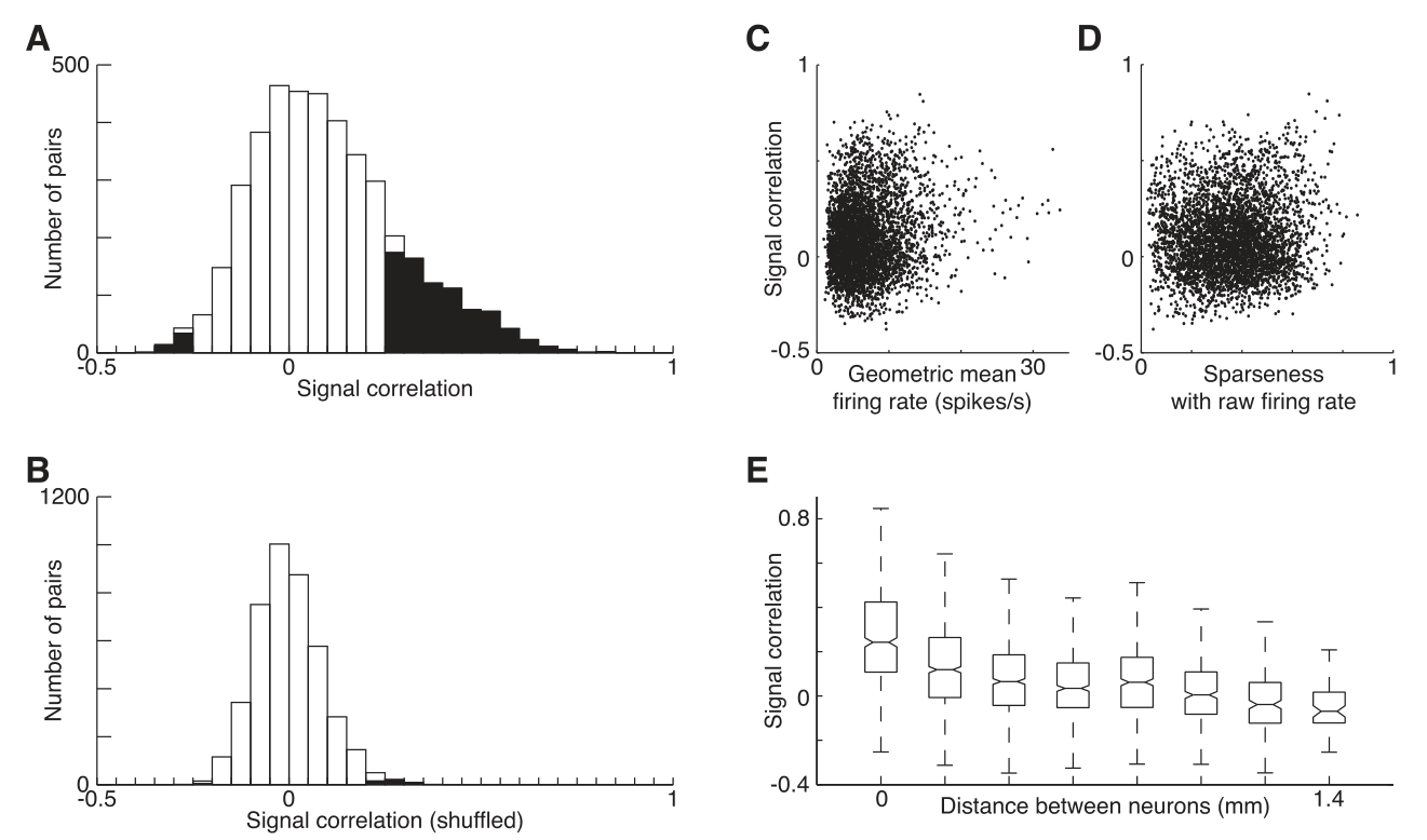
图 6 · 4191 对神经元的 noise correlation

原文图注：Fig. 6. Noise correlation of 4,191 IT neuron pairs within 1.4 mm of each other. A: frequency distribution of the noise correlations. Filled column, significant correlation (P < 0.01, test for independence). Open column, nonsignificant correlation. B: relationship between firing rate and noise correlation. C: relationship between sparseness and noise correlation. D: relationship between noise correlation and neuron distance. We divided neuron pairs into eight groups according to the distance between the neurons: 0 mm (n = 565), 0.2 mm (n = 962), 0.4 mm (n = 841), 0.6 mm (n = 599), 0.8 mm (n = 550), 1.0 mm (n = 382), 1.2 mm (n = 222), and 1.4 mm (n = 70). Other aspects of the figure are as described for Fig. 5.

读法：与图 5 完全平行的一套分析，但对象换成单试次响应波动。整体中位 0.02（35% 的对显著为正）；与放电率弱正相关（r=0.19）、与 sparseness 弱负相关（r=−0.13）；D 面板显示距离梯度同样陡峭——相邻对中位 0.09，0.4 mm 起即不足 0.025（Spearman −0.36）。它支撑结果 2 后半部：试次共变的范围比想象中更局部。

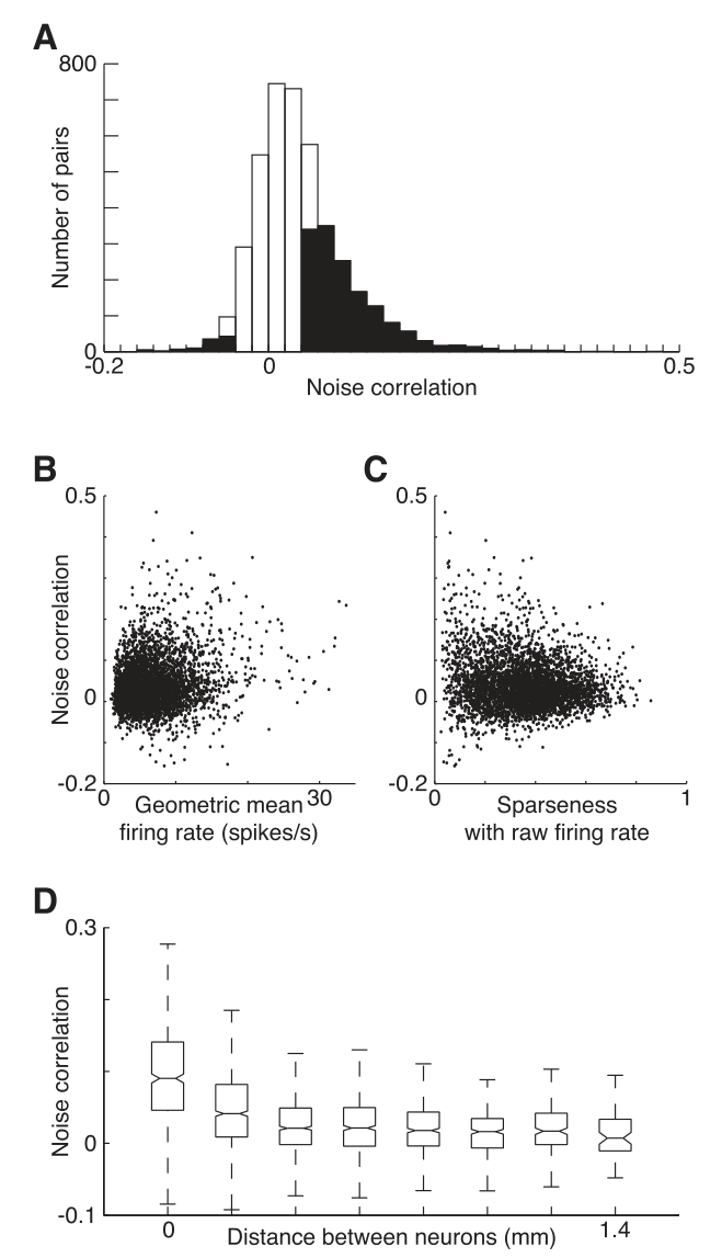
图 7 · CCG 峰的出现概率与强度随距离衰减

原文图注：Fig. 7. Cross correlation of spikes for 4,191 IT-neuron pairs within 1.4 mm of each other. A and B: frequency distribution of CCG-peak magnitudes for all the pairs (A) and pairs with a significant peak (P < 0.0001; B). The rightmost column included pairs with peak magnitude > 0.025. C: relationship between the probability of a significant CCG peak and neuron distance. D: relationship between CCG-peak magnitude and neuron distance. We divided neuron pairs into eight groups according to the distance between the neurons: 0 mm (n = 565), 0.2 mm (n = 962), 0.4 mm (n = 841), 0.6 mm (n = 599), 0.8 mm (n = 550), 1.0 mm (n = 382), 1.2 mm (n = 222), and 1.4 mm (n = 70). Other aspects of the figure are as described for Fig. 5.

读法：A、B 分别给出全部对与有显著峰对的峰高分布（后者中位 0.0070）；C 是出现概率对距离的曲线——从相邻对的 46% 跌至 0.2 mm 的 24%、0.4 mm 起不超过 11%；D 是峰高对距离的箱线图（相邻对 0.0048，0.4 mm 起 ≤0.003）。这张图支撑结果 1，确立了"IT 的毫秒级功能交互以局部为主"的基本事实。

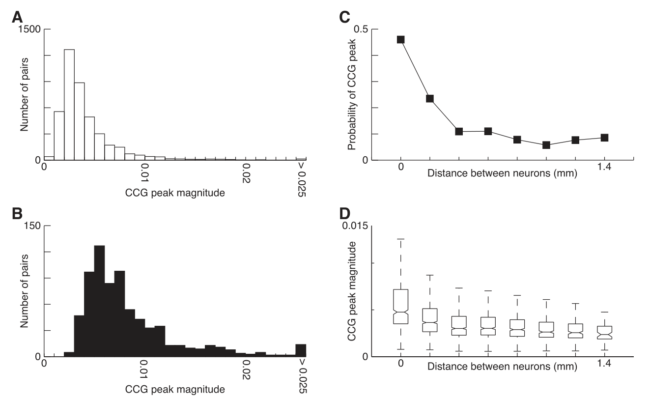
图 8 · 峰高与 signal/noise correlation 的总体关系

原文图注：Fig. 8. Relationships between CCG-peak magnitude and the degree of signal (A) or noise (B) correlation. Bin width, 0.03 for signal correlation, 0.014 for noise correlation; CCG-peak magnitude was plotted in a logarithmic scale. Number of pairs are plotted with a color scale.

读法：两张二维色图，横轴分别为 signal correlation（组距 0.03）与 noise correlation（组距 0.014），纵轴为对数坐标的 CCG 峰高，颜色表示每格内的对数。CCG 峰高随 signal correlation 增大而增大（整体 r=0.31），随 noise correlation 增大的关系更强（r=0.50）——后者在理论上是必然的（noise correlation 与 CCG 曲线下面积相关），作者明言这是确证性而非独立发现。它支撑结果 3 的总体形式。

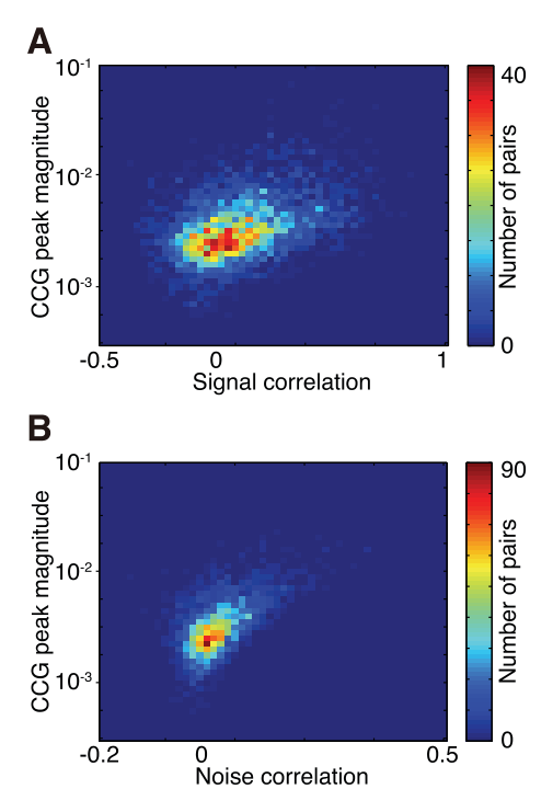
图 9 · 峰参数、距离与相关程度的三元关系

原文图注：Fig. 9. Relationships among CCG-peak parameters, neuron distance, and the degree of signal or noise correlation. A and B: relationship among probability of a significant CCG peak (A) or CCG-peak magnitude (B), neuron distance, and degree of signal correlation. C: the number of neurons contributing to each bin for signal correlation analysis. D and E: relationship among probability of a significant CCG peak (D) or CCG-peak magnitude (E), neuron distance, and degree of noise correlation. F: the number of neurons contributing to each bin for noise correlation analysis. Probability of peak (A and D) and peak magnitude (B and E) are plotted with a color scale. CCG-peak magnitude is the median peak magnitude across neuron pairs in a combination of distance and binned correlation values. Distance between neurons is plotted on the horizontal axis, and degree of signal (A and B) or noise (D and E) correlation is plotted on the vertical axis……

读法：这是图 8 的二维升级版：横轴换成神经元距离，纵轴换成分组后的 signal（A、B）或 noise（D、E）correlation，色标分别是显著峰的出现概率与峰高中位数，C、F 给每格的实际对数（少于 4 对的格子涂黑、不纳入解读）。图上最亮的一角是"距离 0 且相关程度高"的组合——signal correlation 高（0.65–0.75）的相邻对 70% 有显著峰、峰高 0.011；noise correlation 高（0.25–0.35）的相邻对概率达 100%、峰高 0.016。它把结果 3 的联合结构完整呈现出来。

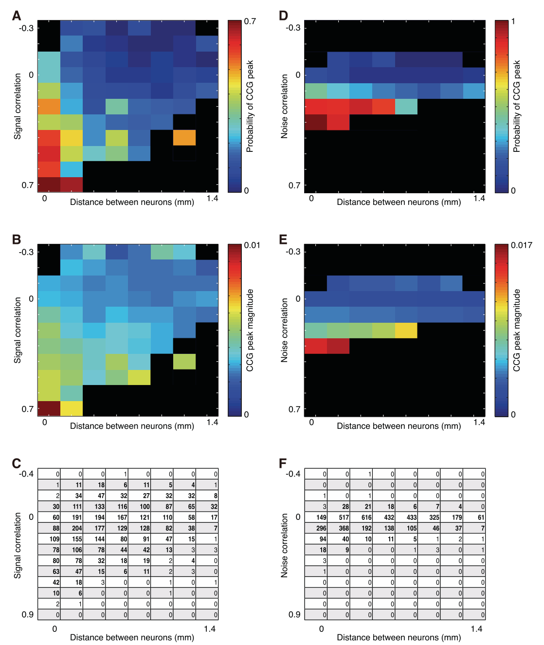
图 10 · 相似性约束随距离增强

原文图注：Fig. 10. Relationships between CCG-peak magnitude and degree of signal or noise correlation for each distance group. A and B: relationships between CCG-peak magnitude and signal correlation for adjacent pairs (distance, 0 mm; A) and for the most distant pairs (distance, 1.4 mm; B). Correlation coefficients (r) between CCG peak magnitude and signal correlation are shown in the plots. C: relationship between neuron distances and correlation coefficients between CCG-peak magnitude and signal correlation. We divided neuron pairs into eight groups according to the distance between the neurons: 0 mm (n = 565), 0.2 mm (n = 962), 0.4 mm (n = 841), 0.6 mm (n = 599), 0.8 mm (n = 550), 1.0 mm (n = 382), 1.2 mm (n = 222), and 1.4 mm (n = 70). Asterisks indicate significant differences between the……

读法：A、B 直接对比两个极端距离组内"峰高 vs signal correlation"的散点：相邻组的相关系数只有 0.23，1.4 mm 组高达 0.70；C 把八个距离组的相关系数连成一条随距离上升的曲线（星号标出与 0 mm 组的显著差异）；D–F 是对 noise correlation 的平行分析（0.46 对 0.81）。这张图支撑结果 4——全文最核心的发现：偏好相似性对连接强度的约束在远距离对之间反而更紧，说明不同距离尺度的连接遵循不同的组织逻辑。

讨论

作者把三组发现归拢为一个组织原理："IT 皮层的水平功能连接同时依据皮层距离与偏好相似性来组织，且距离越远、功能约束越强。"强局部交互与解剖基础吻合——相邻 IT 神经元的基树突野在 0.4 mm 范围重叠，天然共享输入；而远至 1.4 mm 仍有弱交互，最可能是发达的水平轴突在介导（IT 的水平轴突横跨约 8 mm，V1 中甚至可以传播 10 mm 以上），1.4 mm 只是本电极阵列的测量上限、不是交互的边界——此前的 IT 连接研究只看过 0.5 mm 以内的对，这一步扩展本身就是贡献。

功能意义的推测落在两个方向上：相邻但偏好不同（或弱相关）的神经元之间的局部交互可能服务于特征捆绑（feature binding），把同物体上不同特征的信号绑在一起，也可参与生成输入信号未显式编码的复杂形状选择性（作者举了"上"形与"T"形共享竖直条输入的例子）；而偏好相似的远距离神经元之间的交互经汇聚或正反馈，可以进一步精炼刺激选择性。作者还逐一排查了"峰高–noise correlation 相关随距离增强"的技术性解释（峰分选的 0 ms bin 低估、CCG 形状、峰电位样本数、对数差异），结论是技术限制不足以解释趋势。不过文中也承认两点局限：本记录在麻醉条件下进行，麻醉与注意状态对相关程度的影响需要未来实验澄清；相邻对 0 ms bin 的欠计数无法完全排除——尽管非相邻短距离对呈现同样趋势、支持发现的稳健性。

一句话总结

这篇笔记我最想留住的画面是图 10 那条把八个距离组串起来的曲线：连接的"功能特异性"不是均匀的，相邻神经元似乎默认兜底式地连着，局部交互承担捆绑与组合之类的杂务，而远距离连接只在偏好彼此匹配的神经元之间幸存，像一条经过精确挑选的长途专线。换句话说，IT 皮层的水平回路在两个尺度上写着两套组织章程——这是我的理解，文中作者只到"不同距离的回路有独特功能"为止，尚未在行为层面验证哪种交互服务哪种计算。

审校与证据追溯 (Verification & Evidence)

图表审计结果

• Fig1: 提取质量 good，对齐度 full，识别面板 [A, B, C, D, E]
• Fig10: 提取质量 good，对齐度 full，识别面板 [A, B, C]
• Fig2: 提取质量 good，对齐度 full，识别面板 [A, B]
• Fig3: 提取质量 good，对齐度 full，识别面板 [A, B, C, D, E, F]
• Fig4: 提取质量 good，对齐度 full，识别面板 [A, B, C]
• Fig5: 提取质量 good，对齐度 full，识别面板 [A, B, C, D, E]
• Fig6: 提取质量 good，对齐度 full，识别面板 [A, B, C, D]
• Fig7: 提取质量 good，对齐度 full，识别面板 [A, B, C, D]
• Fig8: 提取质量 good，对齐度 full，识别面板 [A, B]
• Fig9: 提取质量 good，对齐度 full，识别面板 [A, B, C, D, E, F]

关键事实与局限性声明

• 审校纠偏: {'overclaim_id': 'OVERCLAIM_001', 'classification': 'OVERCLAIM', 'md_section': '一句话定位', 'current_text': '不同距离尺度的连接承担不同功能——这直接关系到物体表征如何在局部组合与长程整合之间分工。', 'problem': '实验没有测量局部组合、长程整合或行为功能。不同距离回路可能具有不同功能是作者的INTERPRETATION，不是直接结果。', 'recommended_fix': '改为：距离相关的功能交互差异提示不同空间尺度的回路可能具有不同组织方式及计算作用，但具体功能尚未得到行为或因果验证。'} -> 评注:
• 审校纠偏: {'overclaim_id': 'OVERCLAIM_002', 'classification': 'OVERCLAIM', 'md_section': '主要结果', 'current_text': '作者据此断定差异来源于底层神经回路本身。', 'problem': '原文仅称该差异“likely to derive from differences in underlying neural circuitries”，且保留同轴spike-sorting限制。中文“断定”错误提升了确定性。', 'recommended_fix': '改为：作者认为该差异更可能反映底层回路差异，但这一解释仍非因果证明。'} -> 评注:
• 审校纠偏: {'overclaim_id': 'OVERCLAIM_003', 'classification': 'OVERCLAIM', 'md_section': '一句话总结', 'current_text': '相邻神经元似乎默认兜底式地连着，而远距离连接只在偏好彼此匹配的神经元之间幸存。', 'problem': '只有46%的相邻对出现显著CCG峰，并非默认连接；远距离组也没有证据证明交互只存在于偏好匹配的神经元之间。“连着”和“幸存”还暗示直接结构连接及选择性保留过程，均未被测量。', 'recommended_fix': '改为：相邻对更常出现且具有更强的CCG峰；在最远的1.4 mm组中，峰高与刺激偏好相似性的相关性高于相邻组。'} -> 评注:
• 审校纠偏: {'overclaim_id': 'OVERCLAIM_004', 'classification': 'INTERPRETATION', 'md_section': '讨论', 'current_text': '局部交互承担特征捆绑与组合，而远距离交互进一步精炼刺激选择性。', 'problem': '这是作者提出的候选功能解释，并未由本研究直接操控或验证。V0讨论段使用了“推测”和“可能”，基本合格，但开头及总结把它升级成了事实性分工。', 'recommended_fix': '仅在讨论中保留，并明确标注为作者推测；不要用它概括主要结果。'} -> 评注:
• 补充要点: : (第 3 页)
• 补充要点: : (第 4 页)
• 补充要点: : (第 10 页)