IT Literature Intelligence 终审版本 (VERIFIED) 论文编号:
106| 原始基线:V0_ZCODE_BASELINE| 语义审核:pass| 图表审核:pass
Rapid invariant encoding of scene layout in human OPA
Henriksson · Neuron · 2019 · Zotero itemID=1095
这篇文章问的是"我们对身边环境几何的一瞬即得的直觉从何而来":作者构造了 32 种房间布局 × 3 种表面纹理 = 96 个系统化场景刺激,用 fMRI 与 MEG 同时测量发现,场景响应区 OPA 的响应模式编码布局且对表面纹理变化保持不变,而删去'比被试眼动和行为都早得多',或明确标注为解读者的推理而非论文结论,例如:'在刺激呈现后约 100 ms 内即已形成,提示前馈计算即可完成'。。它与海马旁回位置区(PPA)形成鲜明对照(PPA 更擅长解码纹理而非布局),为"OPA 是环境几何的皮层表征所在"提供了最直接的一组证据。
研究背景
成功的空间导航需要大脑表征局部环境的几何——墙壁这样的边界约束可行走的路径,是环境几何的核心成分;甚至幼童在重新定向时也会自动利用房间几何。在皮层端,人类已知有三个对场景图片优先响应的脑区:PPA(parahippocampal place area,海马旁回位置区)、OPA(occipital place area,枕叶位置区)与 RSC(retrosplenial cortex,压后皮层)。早期 fMRI 研究已发现驱动这些场景选择性脑区的是空间布局而非场景内具体物体,后来又有研究区分开阔与封闭场景、关注边界的垂直高度。已有的 functional 证据还提示 OPA 编码场景中可通行的路径(Bonner 和 Epstein 2017),用经颅磁刺激暂时扰乱 OPA 会损害人在导航任务中利用边界的能力(Julian 等 2016)。
但缺口在于具体机制层面:这些场景区究竟如何表征局部环境的几何——尤其是,是否存在一个对表面外观(texture)不变、只关于空间结构的显式布局表征?以往刺激集多取自然照片,低级图像特征与三維几何相互纠缠,无法回答"哪个脑区编码的是几何本身而非图像统计"。此外,布局表征的时间进程(是前馈计算就能完成,还是需要反复加工)在 2019 年之前也缺乏直接测量。这正是本文要填补的两块空白。
研究思路
作者的核心策略是"完备 stimulus 空间 + 双模态成像 + 模型比较"。刺激端用 3D 建模软件(Blender)构造一个系统化集合:五个场景边界元素(左墙、后墙、右墙、地板、天花板)逐一开关,得到 2⁵ = 32 种全部可能的布局,再以三种表面纹理(空房间、栅栏、城市空间)渲染成 96 张图像。完备集合的好处有三:布局与纹理两个因素被完全交叉、可以分离;可以通过"在一种纹理上训练线性判别、在另一种纹理上测试"来检验布局表征的纹理不变性(若判别泛化,则低级图像特征差异的混淆即被排除);还可以逐个估计五个边界元素对表征的相对贡献。
测量端同时用 fMRI(毫米级空间分辨率,分辨 V1、OPA、PPA 内部的响应模式)与 MEG(毫秒级时间分辨率,追踪布局编码的涌现动态),两模态用表征不相似性矩阵(representational dissimilarity matrix, RDM)搭桥:先用 Kendall tau-a 等级相关检验 MEG 时间进程上的 RDM 能被哪个 fMRI ROI 的 RDM 解释,再用一组相互竞争的模型(低级图像特征模型 GIST、等权汉明距离模型、逐元素拟合权重的布局模型、空间开放度模型、元素交互模型)拟合脑与 MEG 的 RDM,找出表征几何的构成。行为端加了一个预先的眼动追踪实验,考察自由观看时被试对场景各部位的注视偏好。
方法
被试共 22 名健康志愿者(9 名女性,平均年龄 26 岁,19–49 岁),每人完成眼动行为实验、一次 MEG 实验和分两次进行的 fMRI 实验(另招募 2 人因未完成两模态实验被排除)。fMRI 在 3T Siemens Skyra 上采集(EPI,TR 2 s,29 层 2 mm,FOV 192 mm,矩阵 96×96),采用快速事件相关设计:刺激图像呈现 2 s、随后仅注视十字 2 s;每次 run 中 96 张刺激各出现一次,混入 32 个 4 s 静息试与 10 个任务试(刺激后偶见指向五个方向之一的箭头,被试按键回答先前布局中该方向是否有边界元素),共 12 个 run(每刺激 12 试)、跨两次测量。以注视点为中心,刺激约占 20°×20° 视野。ROI 界定独立于主实验:V1 依据皮层沟回(Freesurfer 表面图谱对齐);OPA、PPA、RSC 依据独立定位实验(场景/面孔/物体/打碎纹理区组刺激,做 one-back 任务),按"场景>面孔"对比手工勾画,左、右半球的体素拼接后分析。
fMRI 分析:对每对布局刺激,Fisher 线性判别在一半 run 上训练、另一半上测试(split-half 交叉验证),得到线性判别 t 值(LDt,可理解为交叉验证、归一化的马氏距离);逐被试计算后汇总 22 人,32 个布局共 496 个两两比较以 FDR 控制。跨纹理泛化即"甲纹理训练、乙纹理测试"。MEG 在磁屏蔽室内用 306 通道全头系统记录(分析仅用 204 个梯度计,采样 1000 Hz,MaxFilter 时空信号空间分离 + ICA 眨眼矫正),改为'单试次响应基线校正(−200–0 ms)'。、45 Hz 低通;刺激呈现 1 s、ISI 2 s,共 8 个 run(每刺激 8 试)。MEG RDM 用留一法交叉验证的马氏距离(LDC)逐时间点构建,与 fMRI RDM(或模型 RDM)以 Kendall tau-a 比较,跨被试做双侧符号秩检验并 FDR 校正。模型拟合用非负最小二乘,权重按留一被试交叉验证。
主要结果
-
OPA 解码布局优于纹理,V1 与 PPA 恰好相反。对所有"同纹理不同布局"的场景对(布局解码)与"同布局不同纹理"的场景对(纹理解码)平均 LDt:V1 与 PPA 都是纹理解码更好;OPA 则是布局解码更好(图 2)。另外,PPA 对"布局纹理都不同"的场景对的判别力系统地高于"仅布局不同"的对子——纹理定义场景身份,提示 PPA 从事的是基于纹理的场景归类而非布局表征。
-
OPA 的布局判别跨纹理泛化,V1 与 PPA 不能。V1 中不同布局确实诱发不同的响应模式,但判别器换一种纹理测试即失败,说明其判别力来自同纹理布局之间的低级图像特征混淆;OPA 的判别器则跨纹理成功泛化,支持"纹理不变的布局表征";PPA 虽对刺激有响应且平均布局判别高于机会,但大多数布局对的模式差异不可靠(图 3C、图 4)。汇总 RDM 与 MDS 可视化还显示:后墙在三个区都对模式区分性影响最强(它覆盖视野更大、居注视中心),在 OPA 中仅天花板有无差异的场景对响应模式相似(天花板贡献弱),边界元素数量也影响模式区分度。
-
纹理不变的布局表征在 MEG 中约 100 ms 内涌现。V1 与 OPA 的 fMRI-RDM 都与 MEG RDM 相关;把 MEG RDM 拟合为 V1 与 OPA fMRI-RDM 的线性组合后,OPA 的独特贡献从刺激呈现后 60 ms 起显著、约 100 ms 达峰(双侧符号秩、FDR 0.01)。更关键的是,用"跨纹理泛化的判别结果"构建的 RDM 里,只有 OPA(而非 V1 或 PPA)与 MEG 相关——显著自 65 ms 起、约 100 ms 达峰,说明 MEG 看到的正是 OPA 那种表面纹理不变的布局表征,且其计算非常快(图 5B、C)。
-
布局模型对 OPA 表征几何的解释优于 GIST。模型比较(图 6 定义了 ewalls 等权汉明距离、fwalls 逐元素拟合权重、nwalls 空间开放度、GIST 低级特征模型):V1 的 RDM 由 GIST 最好预测;OPA 中 fwalls 显著优于 GIST,再叠加 GIST 反而不增加解释方差(在 V1 中会增加);加入 nwalls 令 OPA 解释方差上升,说明"空间开放度"被编码;PPA 的最佳预测来自 GIST + fwalls + nwalls 的组合,补一句:'交互成分在 V1 与 OPA 中略增解释方差但不达校正后显著,故未纳入完整模型;V1 平均响应强度随纹理细节量递增(空房间 < 栅栏 < 城市)'。。MEG 上,GIST 主导早期表征,但边界元素成分在早期显著附加解释力并在约 100 ms 达峰,nwalls 的附加贡献集中在晚期时间点(图 7)。
-
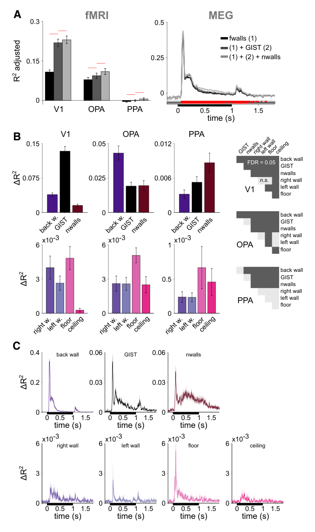
地板在 OPA 表征中地位特殊,与眼动行为一致。逐成分独特方差的"留一"分析显示:GIST 主导 V1;V1 与 OPA 中后墙的贡献都强于其他元素;OPA 里地板的贡献显著大于右墙、左墙与天花板(FDR 0.05),MEG 结果一致。行为端在成像前对 96 张刺激的自由观看中,被试向下视野、尤其是向地板的注视显著多于天花板(每纹理 FDR = 0.0035、0.0077、0.003),提示注意被自动导向脚下的可行走几何(图 8,行为结果见补充材料)。
图注解读
图 1 · 完备的场景布局刺激集
原文图注:Figure 1. Stimuli to Test the Hypothesis that Human Scene-Responsive Cortical Areas Encode Scene Layout (A) The spatial layout of a room is captured by fixed scene-bounding elements, such as the walls. (B) We created a complete set of spatial layouts using 3D modeling software by switching on and off the five bounding elements: left wall, back wall, right wall, floor, and ceiling. (C) For example, by switching off the back wall and the ceiling, we create a long, canyon-like environment. (D) Textures and background images were added to the scenes to enable us to discern layout representations from low-level visual representations. (E) The complete set of scenes included 32 different spatial layouts in 3 different textures, resulting in 96 scene stimuli.
读图要点:(A) 立出"房间布局由固定边界元素定义"的概念;(B) 说明用 3D 建模软件把五个元素逐一开关;(C) 给出实例——关掉后墙与天花板即得到狭长的峡谷式环境;(D) 强调加纹理与背景图像的目的:把布局表征与低级视觉表征区分开;(E) 展示全部 32 布局 × 3 纹理 = 96 张刺激。这张图确立全文最关键的方法学资产——完备 stimulus 空间——支撑结果 1、2 的推理前提。
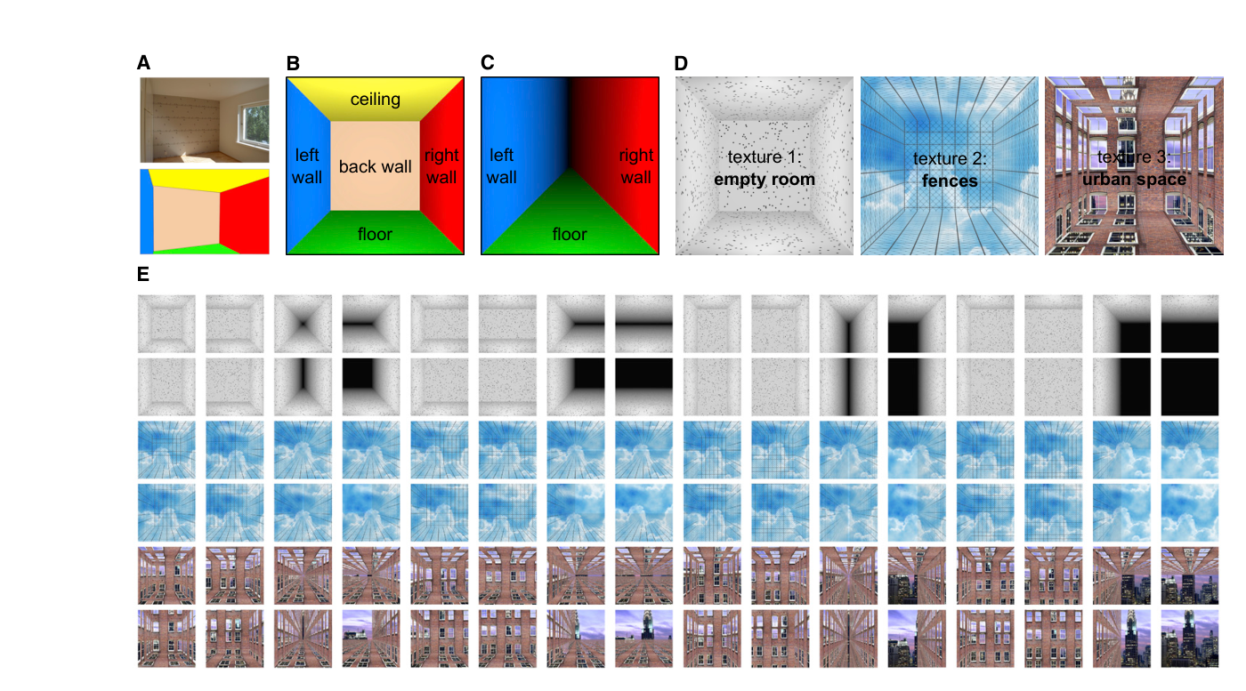
图 2 · 布局解码与纹理解码的对比
原文图注:Figure 2. Layout versus Texture Decoding The average discriminability across all scene pairs that differ in the layout but are of the same texture (layout decoding; gray bars) and all scene pairs that have the same layout but differ in the texture (texture decoding; black bars) are shown separately for the V1, OPA, and PPA. In the V1 and PPA, a change in texture had, on average, a larger effect on the discriminability of the fMRI response patterns than a change in layout, whereas the opposite was true for the OPA. The p values are from two-tailed signed-rank tests across the 22 subjects; the error bars indicate SEM across the subjects. See Figure S1 for average fMRI responses for all 96 individual stimuli for each region of interest and Figure S2 for fMRI response pattern discriminability separately for each stimulus pair.
读图要点:x 轴为 V1、OPA、PPA 三个 ROI,y 轴为平均判别力(LDt);灰色柱是布局解码(同纹理、不同布局的场景对平均),黑色柱是纹理解码(同布局、不同纹理的场景对平均),误差棒为跨 22 名被试的 SEM,p 值来自双侧符号秩检验。读图口诀是看两柱的相对高低:V1 与 PPA 黑柱高(纹理带来的模式差异更大),OPA 灰柱高(布局差异更大且高于纹理差异)。这是全文的第一个分离性结果,支撑结果 1。
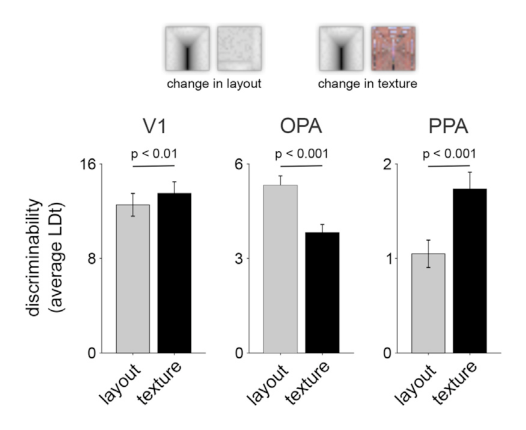
图 3 · 布局判别的跨纹理泛化检验
原文图注:Figure 3. Discriminability of the fMRI Response Patterns for Each Pair of Layout Stimuli in the V1, OPA, and PPA and Generalization of the Result across Textures (A) The discriminability of the layout stimuli from the fMRI response patterns was evaluated for each pair of the 32 layouts, separately for the three textures. The Fisher linear discriminant was fitted to response-patterns obtained from training data (odd fMRI runs) and the performance was evaluated on independent testing data (even fMRI runs). The results are shown as linear discriminant t values (LDt; Nili et al., 2014; Walther et al., 2016). The analyses were done on individual data, and the results were pooled across subjects. (B) The generalization of the layout discrimination across different surface textures was evaluated by fitting the Fisher linear discriminant to response patterns corresponding to a pair of layouts in one texture and evaluating the performance on the response patterns corresponding to the same layout pair in another texture. All combinations of texture pairs were evaluated. A high LDt value suggests successful generalization of layout discrimination across surface textures and, hence, a layout representation that is tolerant to a change in surface texture.
读图要点:(接上文;(C)部分为)上排是 32×32 的 LDt 矩阵:对角线三个矩阵分别是三种纹理内部的布局判别,六个非对角矩阵是跨纹理泛化(一种纹理训练、另一种纹理测试同一布局对);下排是相应的期望假发现率矩阵(n.s. 即不显著)。读法:V1 对角线亮而非对角暗——模式可分但不泛化,即判别力是低级图像特征的混淆;OPA 对角线与非对角都亮——判别力跨纹理保持,支持纹理不变的布局表征;PPA 只有个别格亮,多数布局对分不开。此图是"OPA 编码布局本身"最直接的证据,支撑结果 2。
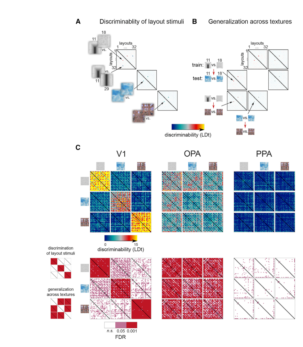
图 4 · 表征几何的汇总:布局泛化在 OPA 成立
原文图注:Figure 4. Representational Geometry of Scene Layouts Generalizes across Textures in the OPA (A) The distinctiveness of the fMRI response patterns for the spatial layouts are shown, as captured by the LDt values. The analyses done separately for the three textures were averaged (shown separately in Figure 3). The bottom row shows the corresponding FDRs (two-tailed signed-rank test across 22 subjects). (B) The generalization performance of the discriminant across different textures was evaluated by fitting the linear discriminant to a pair of spatial layouts in one texture and testing the discriminant on the same pair of layouts in another texture. The analysis was done for each combination of textures, and the results were averaged (shown separately in Figure 3). The bottom row shows the corresponding FDRs. In the OPA, the representation shows texture invariance. The multidimensional scaling visualizations of the distinctiveness of the response patterns are shown in Figure S3.
读图要点:把图 3 的逐纹理结果在 V1、OPA、PPA 三个区取平均成汇总 RDM:(A) 为纹理内判别,(B) 为跨纹理泛化判别,下排均为对应显著性(FDR)矩阵,右侧注色条标 LDt 值高低。读图时注意三个区的对比——V1 的 (B) 明显弱于 (A),OPA 的两者几乎同样亮,PPA 两者都淡;再注意后墙的行/列在各区都偏亮(后墙覆盖视野中心且面积大)。文中还借 MDS 可视化指出 OPA 中仅差天花板的场景对模式相似。此图支撑结果 2 及"后墙主导、天花板贡献弱"的细分观察。
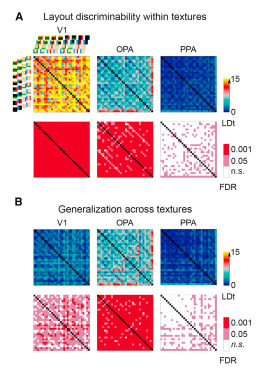
图 5 · OPA 的 fMRI 表征与 MEG 时间动态的早期对应
原文图注:Figure 5. Early Correspondence between the Representations in the OPA (fMRI) and MEG (A) The Kendall tau-a rank correlations between the MEG RDMs and fMRI RDMs are shown. The top panel shows the full time course (stimulus-on period indicated by the black bar), and the bottom panel highlights the early time window. The black line shows the correlation between the MEG and V1-fMRI, and the dark red line shows the correspondence between the MEG and OPA-fMRI. The correspondence between the MEG RDMs and cross-validated fitted linear combinations of multiple fMRI RDMs are also shown (light red line for the V1 and OPA and blue dashed line for the V1, OPA, and PPA). The analyses were done separately for each subject and for each texture, and the results were averaged. Significant time points are indicated by thick lines (FDR of 0.01; p values were computed with two-tailed signed-rank test across the 22 subjects, FDR adjusted across time points). The gray line indicates the amount of replicable structure in the MEG RDMs across subjects. Figure S4 evaluates the effect of the distance estimator for the reliability of the RDMs. (B) The OPA significantly adds to the V1 in explaining the MEG RDMs already in the early time window after stimulus onset. Shaded regions indicate SEM across subjects, and a red line indicates an FDR rate of 0.01
读图要点:(A) 画 MEG RDM 与各 fMRI RDM 的 Kendall tau-a 相关随时间的曲线:黑线为 V1-fMRI、深红线为 OPA-fMRI,浅红线与蓝色虚线分别是 V1+OPA 及 V1+OPA+PPA 的拟合组合,灰色线为 MEG RDM 跨被试的可复制结构,粗线段为 FDR 0.01 校正后的显著时段。(B) 是"把 MEG RDM 拟合为 V1 与 OPA 的线性组合后 OPA 的独特贡献"随时间的曲线:显著起点约 60 ms、峰值约 100 ms,阴影为跨被试 SEM、红线为 FDR 0.01 显著阈。(C) 只画跨纹理泛化 RDM 与 MEG RDM 的相关——仅 OPA 显著(约 65 ms 起、约 100 ms 峰),V1 与 PPA 不显著。此图把空间结论(OPA)与时间结论(约 100 ms 内)焊在一起,支撑结果 3。
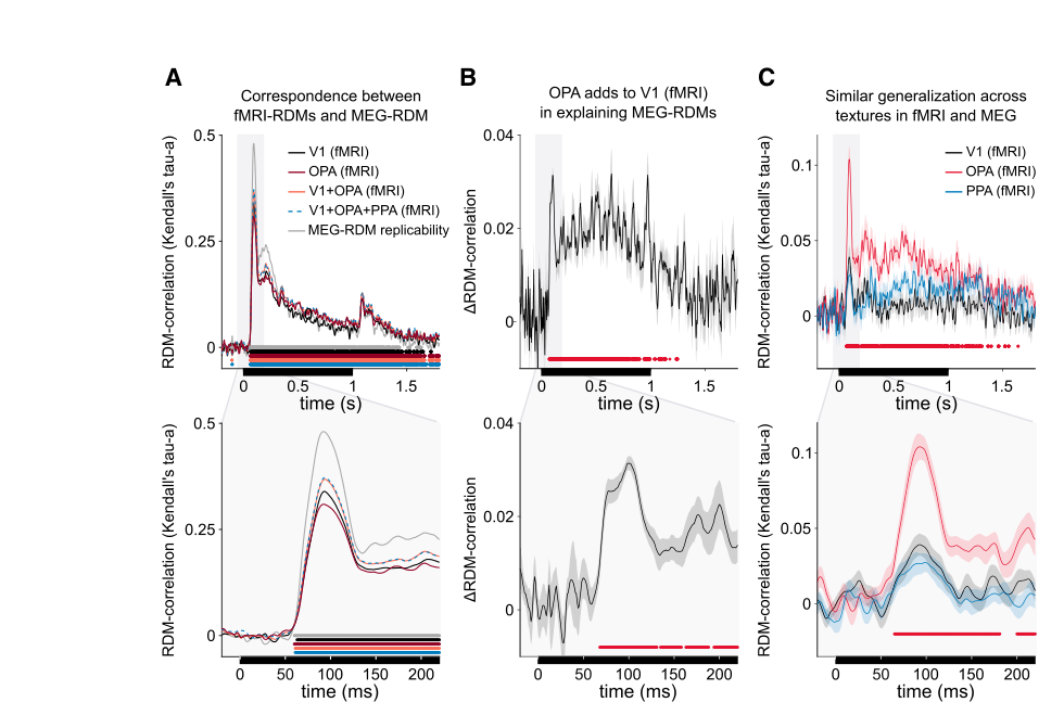
图 6 · 表征几何的模型成分
原文图注:Figure 6. The Representational Geometries Were Modeled as Linear Combinations of Representational Components The first three model-RDMs capture the GIST features (Oliva and Torralba, 2001) of the stimuli (low-level image feature similarity), shown separately for the three different textures. The next model predicts the responses for a scene layout-based representation with equal contribution of all walls, calculated as the Hamming distance between the layouts (the percentage of the same boundaries present in a pair of scenes, predicting a similar response to two scenes with the same boundaries and a distinct response for a pair of scenes with different boundaries). The last model in the top row was constructed based on the number of scene-bounding elements present in each scene (a similar response to a pair of scenes with the same number of scene elements present in the scene), roughly reflecting the size of the space. The center row shows the five model-RDMs separately capturing the presence of each of the five scene-bounding elements in the spatial layouts. The last ten model-RDMs reflect the interactions between the walls.
读图要点:本图不是结果而是模型库清单:排首的是三个逐纹理的 GIST 低级特征 RDM;随后是 ewalls(把五个边界元素等权、用布局间 Hamming 距离计算)与 改为'nwalls(按场景中边界元素的数量预测模式相似性,大致对应空间大小/开放度)'。两个布局模型;中间一行为 fwalls 的五个逐元素 RDM(每个元素一个);底部十个小格是元素两两交互 RDM。它们经非负最小二乘拟合并留一被试交叉验证后与脑 RDM 比较,是图 7、图 8 的输入。读懂这张模型清单,就明白了结果 4 里"fwalls 优于 GIST"等比较分别在比什么。
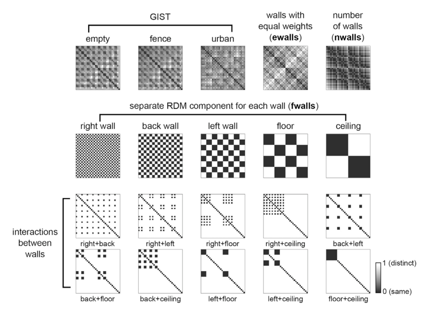
图 7 · 各模型对 fMRI 与 MEG RDM 的解释力
原文图注:Figure 7. The Contributions of Low-Level Image Differences and True Scene Layout-Based Representations in the fMRI and MEG RDMs (A) The mean Kendall's tau-a correlation between the models and fMRI RDMs are shown separately for the V1, OPA, and PPA. In the V1, there is only a small improvement in the correlations when the GIST model is complemented with other models. In the OPA, the fitted combination of scene-bounding elements model (fwalls) alone already explain the representation better than the GIST model. The gray lines indicate the amount of replicable structure in the fMRI RDMs across subjects. The error bars indicate SEM across the subjects. (B) Pairwise comparisons between the models, shown separately for the V1, OPA, and PPA. The color codes and order of the models is the same as in (A). Dark gray indicates a significant difference between the models (two-tailed signed-rank tests across the 22 subjects, multiple testing accounted for by controlling the FDR at 0.01), light gray indicates non-significance.
读图要点:(A) 是七个模型(GIST、nwalls、ewalls、fwalls、GIST+fwalls、GIST+fwalls+nwalls、再+交互)对三个区 fMRI RDM 的平均 Kendall tau-a 相关柱状图,灰线为 RDM 的可复制结构上限。(B) 是模型两两比较矩阵,深灰为 FDR 0.01 下显著、浅灰不显著。读图口诀:V1 一栏 GIST 已接近上限、加布局模型改善很小;OPA 一栏 fwalls 单独就超过 GIST,且 GIST+fwalls 相对 fwalls 无显著增益、加 nwalls 却显著更好;PPA 需要全部成分组合才最佳。(C)–(E) 把同样的比较铺到 MEG 时间轴上:(C) 各模型拟合时间进程(黑框为刺激呈现),(D) fwalls 在 GIST 之上的附加贡献约 100 ms 达峰,(E) nwalls 的附加贡献集中在更晚时段。此图支撑结果 4。
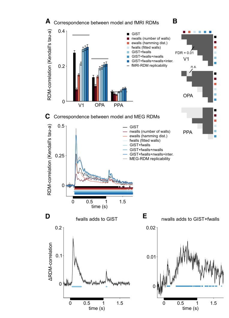
图 8 · 逐成分的独特解释方差
原文图注:Figure 8. The Unique Variance Explained by Each Model Component (A) The explained variance (R2 adjusted) of the fitted joint models containing components for the five scene-bounding elements (black bars and line for fMRI and MEG, respectively), components for the five scene-bounding elements and the GIST (dark gray bars and line), and components for the five scene-bounding elements, the GIST, and the number of walls (light gray bars and line). The red lines indicate a significant improvement compared with a model with fewer components (one-tailed signed-rank tests across the 22 subjects, multiple testing within a region of interest or across time points accounted for by controlling the FDR at 0.05). See Figures S5 and S6 for the results for each texture separately and also including the component models for interactions between walls (overall no further improvement in the adjusted explained variance). (B and C) The gain in variance explained by each of the model components was calculated by comparing the explained variance between the full model (light gray in A) with a model where this one component was left out from the joint fit. Each model component was left out in turn, and the results are shown separately for (B) V1, OPA, and PPA (fMRI) and (C) MEG data. Error bars (fMRI) and shaded regions (MEG) are SEM across subjects.
读图要点:(A) 比较三层嵌套联合模型的校正 R²(仅五个边界元素 / 加 GIST / 再加 nwalls),柱为 fMRI、线为 MEG,红线标出比少成分模型显著改善(FDR 0.05)。(B)、(C) 是"留一成分"分析:从完整模型中逐一去掉每个成分、看解释方差掉多少(ΔR²),(B) 为 V1/OPA/PPA 的 fMRI,(C) 为 MEG。读图要点:GIST 成分在 V1 的 ΔR² 量级远超布局成分;OPA 中后墙分量最大、地板显著大于左右墙与天花板;MEG 与 OPA 一致且地板的突出贡献与行为眼动结果呼应。此图支撑结果 5。
讨论
作者的结论框架是:OPA 从视觉输入中提取场景边界元素的布局,其表征支持对"边界有无"的线性读出、且对表面纹理操作不变;V1 的表征则被 GIST 低级特征模型而非布局模型更好地捕获;PPA 的响应模式不能可靠区分多数布局对,纹理解码反而更好,且"布局纹理都不同>仅布局不同"的模式表明它参与基于纹理的场景归类。这与 Julian 等 2018 的"OPA 分析局部场景元素、PPA 参与场景识别"的分工观一致,也与 OPA 具有下视野/外周视野偏置的报道(Silson 等 2015、Levy 等 2001/2004)互相印证;作者进一步借自家提出的"面孔区拓扑地图假说"(faciotopy)类比:场景响应皮层或许同样从视网膜拓扑原图发育为对行为上最重要特征(如脚下的地面)有放大表征的场景布局图。与 Lescroart 和 Gallant(2019)的计算机生成刺激建模工作对话,作者认为本文的贡献在于 OPA 与 PPA 的表征分离(只有 OPA 表征纹理不变的布局)以及该表征在 MEG 中约 100 ms 的快速涌现——后者支持 Bonner 与 Epstein(2018)的建模结论:布局可以由前馈机制高效算出。作者明确承认的局限包括:用的是 2D 渲染而非 3D/VR 呈现;为保持刺激完备性,各布局的出现等概率,未区分自然常见与罕见布局;纹理只有三种,一些与布局共变的知觉差异(如知觉距离)尚未完全解开,后墙的贡献也可能混入"移除后墙增加场景深度"的效应;地板的特殊地位究竟是"地面几何本身"还是"下视野加工偏置"也有待未来的工作厘清。
一句话总结
这篇论文是我心中"用完备 stimulus 空间撬开一个问题"的典范之作:交叉化设计使纹理不变性变成可检验的泛化事实,fMRI-RDM 与 MEG 时间进程的搭桥又把"在哪里"和"何时"缝进同一张表征之网。以我的理解,最值得玩味的是它逼着 PPA 让位——"场景区"不是一个东西,看布局的 OPA 与认场景的 PPA 在功能上是两套算法。
审校与证据追溯 (Verification & Evidence)
图表审计结果
- Fig1: 提取质量
good,对齐度full,识别面板[A, B, C, D, E] - Fig2: 提取质量
good,对齐度full,识别面板[] - Fig3: 提取质量
good,对齐度full,识别面板[] - Fig4: 提取质量
good,对齐度full,识别面板[] - Fig5: 提取质量
good,对齐度full,识别面板[] - Fig6: 提取质量
good,对齐度full,识别面板[] - Fig7: 提取质量
good,对齐度full,识别面板[] - Fig8: 提取质量
good,对齐度full,识别面板[A]
关键事实与局限性声明
- 审校纠偏: 开篇'比被试眼动和行为都早得多':原文无此比较,属解读者推断(ISSUE_001)
- 审校纠偏: 开篇'用 fMRI 与 MEG 同时测量':'同时'易被误读为同步采集,实际 fMRI 与 MEG 为分开的实验session(fMRI 还分两次),建议改为'分别用 fMRI 与 MEG 测量'
- 补充要点: RSC 负结果:多数刺激未在 RSC 诱发可测量响应,RSC 仅出现在补充材料(见 ISSUE_004)
- 补充要点: V1 单变量响应强度受纹理调制(empty < fence < urban),反映低级图像细节量,是其模式可分性来自低级特征的旁证
- 补充要点: fMRI/MEG 实验期间在线眼动追踪用于监控中央注视稳定性(STAR Methods),可作为'结果不受眼动混淆'的控制说明
- 补充要点: 任务试在 MEG 中以抬指(finger lift)作答、fMRI 中以按键作答——解读未区分两模态的作答方式,但不影响结论