IT Literature Intelligence 终审版本 (VERIFIED) 论文编号:
104| 原始基线:V0_ZCODE_BASELINE| 语义审核:pass| 图表审核:passAstra裁决:compromise_revision(revise)
Evidence that recurrent circuits are critical to the ventral stream's execution of core object recognition behavior
Kar · Nature Neuroscience · 2019 · Zotero itemID=1082
这是一篇用"行为筛选 + 大规模电生理 + 深度网络建模"三方联动的实证研究:作者先找出灵长类能轻松识别、但纯前馈深度卷积神经网络解不出的"挑战图像",再用 Utah 阵列记录猕猴下颞叶(IT)皮层群体活动,发现这些图像的"行为充分"物体信息在 IT 中平均晚约 30 ms 才解出,且这一晚期响应模式恰好是前馈网络预测最差的部分。它把"循环回路(recurrent circuits)对快速物体识别是否必要"这一长期悬而未决的问题变成了可定量检验的命题,也给了后续循环神经网络模型一组明确的约束条件,因此是这个方向绕不开的标志性工作。
研究背景
灵长类在一次约 200 ms 的注视内就能完成对中心视野物体的快速识别,即所谓核心物体识别(core object recognition)。此前研究已知,物体身份明确地编码在猕猴下颞叶皮层(inferior temporal cortex, IT)的群体活动模式中,而目前最能同时预测 IT 单细胞响应和灵长类行为的模型,是在 ImageNet 上做物体分类训练的深度卷积神经网络(deep convolutional neural network, DCNN)。问题在于:这类模型几乎是纯前馈(feedforward)的,而真实腹侧视觉通路却布满皮层间、皮层下及区内长程的循环连接。由于 200 ms 的窗口很短,一种流行的假说是核心物体识别根本不需要循环计算——循环回路或许只在更慢的时间尺度上(比如突触可塑性)起作用。这篇文章的首要目标就是尝试证伪这个假说。
当时的缺口有两处。其一,虽然不断有报道称前馈 DCNN 在某些图像上无法准确预测灵长类行为,但没有人系统地、图像逐一比对地找出"模型失败而灵长类成功"的具体图像,并把它们当作探针去追踪神经机制;以往对反馈作用的讨论多停留在"遮挡、杂乱、分组"这类单一名词化的图像属性上,缺乏图像可计算、行为相关的操作性定义。其二,IT 群体解码的时间动态虽然有人测过,但以往工作使用的解码时间窗较宽,无法精确刻画每张图像的"解出时刻",因而也无法检验"循环依赖的图像需要额外加工时间"这一关键预测。
研究思路
作者的总体策略是一个三段论式的逻辑链。第一,如果循环计算对核心识别行为是关键的,那么必然存在一些图像:前馈网络(作为腹侧流前馈通路的函数近似)解不出,而灵长类轻松解决——这样的图像最可能受益于循环计算。为避免对图像类型(遮挡?杂乱?模糊?)先入为主,作者采用数据驱动的方式,用二元物体辨别任务逐图像比较猕猴、人类与 AlexNet fc7 的行为表现,筛出"挑战图像"(challenge images)与"对照图像"(control images)两组。第二,如果这些图像确实依赖循环计算,其循环影响应体现在图像驱动的 IT 响应晚期,那么挑战图像在 IT 中达到"与行为同样好"的线性解码水平就应该更晚。第三,反过来,那些行为上起关键作用的晚期 IT 响应模式,应该让前馈模型预测失灵,而带循环或等效深度的模型预测更好——这构成对模型端的检验与约束。
这个设计的巧妙之处在于把"循环是否参与"翻译成了两个可测量的量:其一,每张图像的物体解出时间(object solution time, OST),定义为 IT 群体线性解码准确率达到该图像上猴子行为准确率水平的时刻;其二,模型对 IT 响应的解释方差随时间的变化。两者都与行为挂钩(OST 以行为准确率为锚),从而避免"晚期响应只是附带现象"的质疑。
方法
行为端:共 1,320 张测试图像(其中 1,120 张为合成"自然图像",10 个物体类别——熊、大象、人脸、苹果、汽车、狗、椅子、飞机、鸟、斑马——各 112 张,通过位置、旋转、尺寸等视角变化生成;另 200 张来自 COCO 数据集的照片,含遮挡、形变、杂乱背景等)。二元辨别任务流程为注视 300 ms 后呈现测试图像 100 ms(视角 8°),空屏 100 ms,然后呈现目标物体与九个干扰物之一的规范视图,人类点击选择、猕猴用眼动选择。人类被试 88 名(Amazon MTurk 平台,每张图像 80 份独立反应),猕猴 2 只(同步做电生理记录)。行为指标 I1 为逐图像的一对多信号检测敏感度 d′(把含某目标的图像与所有其他物体的图像区分开的辨别力),人类与猕猴的 I1 分半信度分别达 0.84 和 0.88。与 AlexNet fc7 逐图像比较后定义:灵长类与模型 d′ 差不超过 0.4 的为对照图像(149 张),灵长类至少高出 1.5 d′ 的为挑战图像(266 张)。
神经端与模型端:两只猕猴 IT 皮层(后、中、前段 PIT/CIT/AIT)各植入多组 10×10 Utah 阵列,共 424 个有效位点,同时在一侧半球记录上游 V4(95 与 56 个位点)。测试图像呈现 100 ms,以多单位活动(multiunit activity)计数,按刺激起点后每 10 ms 非重叠时间窗构建群体活动向量;对每个时间窗独立训练和交叉检验线性 SVM 解码器,得到逐图像的神经解码准确率(neural decoding accuracy, NDA)随时间的轨迹,再用非线性拟合确定 NDA 达到猴子行为 d′ 误差范围的时刻,即该图像的 OST(经 bootstrap 估计平均标准误约 9 ms)。模型端用各 DCNN 的特征(投影到前 1,000 个主成分)以偏最小二乘回归逐位点预测 IT 响应,计算经噪声校正的解释方差百分比(IT predictivity);另测试了带区内循环连接的四层循环网络 CORnet(IT 层迭代 5 个时间步)。此外还做了后向掩蔽实验(见下)与多组控制分析。
主要结果
-
逐图像行为比较成功筛出两组图像,且灵长类反应时更长。平均而言猕猴和人类都优于 AlexNet;对照与挑战图像分别有 149 与 266 张。两类图像在视觉检查上没有可分辨的单一图像属性差异,重复接触也不改变表现,但挑战图像的反应时显著更长(猕猴 ΔRT = 11.9 ms,t(413) = 3.4,P < 0.0001;人类 ΔRT = 25 ms,t(413) = 7.52,P < 0.0001),提示其确实需要额外加工时间(图 1d,e)。
-
挑战图像的 IT 解出时间平均晚约 30 ms。约 91% 的挑战图像与 97% 的对照图像的 IT 解码最终都能达到灵长类行为水平;但 OST 中位数分别为 145 ± 1.4 ms 与 115 ± 1.4 ms,相差约 30 ms(图 2c)。用一半位点重估 OST 与全体位点高度相关(Spearman R = 0.77/0.76),且 ΔOST 保持在约 30 ms,说明估计稳健。
-
该滞后不能归因于视觉驱动变慢或低级图像属性。两组图像的 IT 群体起始潜伏期差仅 0.17 ± 0.21 ms(P = 0.69),V4 的起始与峰值潜伏期也无差异(t(150) = 0.2,P = 0.8);图像的起始潜伏期与 OST 完全不相关(r = 0.009,P = 0.8),有的挑战图像 IT 起始反应很快(早于平均)却解出很慢(约 200 ms)。事实上挑战图像在约 150 ms 处的群体发放率反而更高(ΔR = 17.3%,P < 0.0001),作者推测这是循环输入的额外驱动。SHINE 低级属性均衡化后 ΔOST 仍有约 24 ms;对比度、模糊、杂乱等属性只能解释 OST 的绝对值而不能解释 ΔOST;高、低潜伏期神经元亚群分别给出约 18 与 22 ms 的解码滞后;被动观看下滞后仍有约 28 ms(与主动任务状态相关 ρ = 0.76),未受训的猴子数据中也存在约 34 ms 的滞后(图 3)。
-
前馈模型恰好对行为关键的晚期 IT 响应预测失灵,更深和循环模型更好。AlexNet fc7 在早期响应段(90–110 ms)可解释 44.3 ± 0.7% 的可解释方差,但随响应演化在 150–200 ms 段跌至 20% 以下;该下降的时间点与挑战图像 OST 的分布吻合。更深的 CNN(Inception-v3/v4、ResNet-50/101)在晚期段的 IT predictivity 比 8 层的"深"模型(AlexNet、Zeiler-Fergus、VGG-S)高 5.8%(t(423) = 14.26,P < 0.0001),带循环的 CORnet 更高,且其第 3、4 遍迭代对晚期响应的预测显著优于第 1、2 遍,与早期正好相反(图 4a,b)。此外,以每个模型自身定义的"挑战图像"看,更深的模型剩下的未解图像在 IT 中需要更长的 OST,暗示它们只部分、隐式地实现了部分循环计算(图 4c)。
-
结果5标题改为『后向掩蔽实验为循环加工对挑战图像识别的重要作用提供行为层面的收敛证据』。正文括号『破坏再入式加工』改为『依据前人研究,后向掩蔽可能干扰再入式加工』。图5读图要点末句改为『结合电生理结果,这为快速循环计算对挑战图像识别的重要作用提供了收敛证据,但尚未直接证明晚期IT响应的必要性。』。在测试图像后立即呈现 500 ms 相位打乱的掩蔽图像(破坏再入式加工),掩蔽对挑战图像的行为损伤显著大于对照图像:图像呈现 34–167 ms 时逐物体平均的控制−挑战 Δd′ 为 0.5、0.81、0.33、0.40(Bonferroni 校正后均显著),而呈现时间延长到约 267 ms 时差异消失(Δd′ = −0.02)。这与"掩蔽限制加工于初始前馈响应、挑战图像恰需要晚期循环加工"的预测一致(图 5)。
-
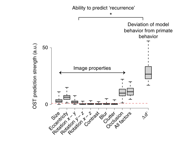
Δd′ 向量是比任何单一图像属性更强的"循环参与度"预测源。物体尺寸、偏心度、遮挡等因素以及全部因素组合对 OST 都只有显著但很弱的预测力,而"AlexNet 与猴子行为之差"(Δd′)对 OST 的预测显著更强(Spearman ρ = 0.44,P < 0.001;组间比较 ANOVA F(1,10) > 100,P < 0.0001,Tukey 检验显示 Δd′ 与所有其他属性都不同)(图 6)。
图注解读
图 1 · 行为筛选:找出挑战图像与对照图像
原文图注:Fig. 1 | Behavioral screening and identification of control and challenge images. a Both primates (humans and macaques) and feedforward DCNNs were tasked to identify which object is present in each test image (1,320 images). Top: the stages in the primate ventral visual pathway (retina, lateral geniculate nucleus (LGN), areas V1, V2, V4, and the IT cortex), which is implicated in core object recognition. We can conceptualize each stage as rapidly transforming the representation of the image and ultimately yielding the primates' behavior (that is, producing a behavioral report of which object was present). The blue arrows indicate the known anatomical feedforward projections from one area to the other. The red arrows indicate the known lateral and top-down recurrent connections. Bottom: a schematic of a similar pathway commonly present in DCNNs. These networks contain a series of convolutional and pooling layers with nonlinear transforms at each stage, followed by fully connected layers (which approximate macaque IT neural responses) that ultimately gives rise to the models' 'behavior'. Note that the DCNNs only have feedforward (blue) connections. b, Illustrations of the ten different object types used in the study. c, Binary object discrimination task, showing the timeline of events for each trial. Subjects fixate on a circle, then the test image at 8° containing one of ten possible objects is shown for 100 ms. After a 100-ms delay, a canonical view of the target object (the same as that presented in the test image) and a distractor object (one of the other nine objects) appears, and the human or monkey indicates which object was present in the test image by clicking on or making a saccade, respectively, to one of the two choices. d, Comparison of monkey performance (pooled across two monkeys) and DCNN performance (AlexNet19 fc7). Each circle represents the behavioral task performance (I1; refer to Methods) for a single image. We reliably identified challenge images (red circles) and control images (blue circles). Error bars are bootstrapped s.e.m. e, Examples of four challenge and four control images.
读图要点:a 面板是全文的概念框架图——上排为灵长类腹流通路(视网膜→LGN→V1→V2→V4→IT),蓝色箭头为前馈投射、红色箭头为横向与自上而下的循环连接;下排是 DCNN 的对应结构,但只有前馈连接(蓝),全连接层被当作 IT 的近似。这一"红箭头缺失"的对比正是全文要检验的假设。c 面板给出任务时间线:注视 300 ms → 测试图像 100 ms → 空屏 100 ms → 选择屏 1,500 ms。d 面板是核心散点图:横轴为 AlexNet fc7 的 d′,纵轴为两只猴子汇总的 d′,每个点是一张图像,蓝点(|d′ 差| ≤ 0.4)落在对角线附近即对照图像,红点(灵长类高出 ≥ 1.5 d′)明显偏离对角线即挑战图像;误差棒为 bootstrap s.e.m.。e 给出两组图像各四个实例。该图支撑上文结果 1。
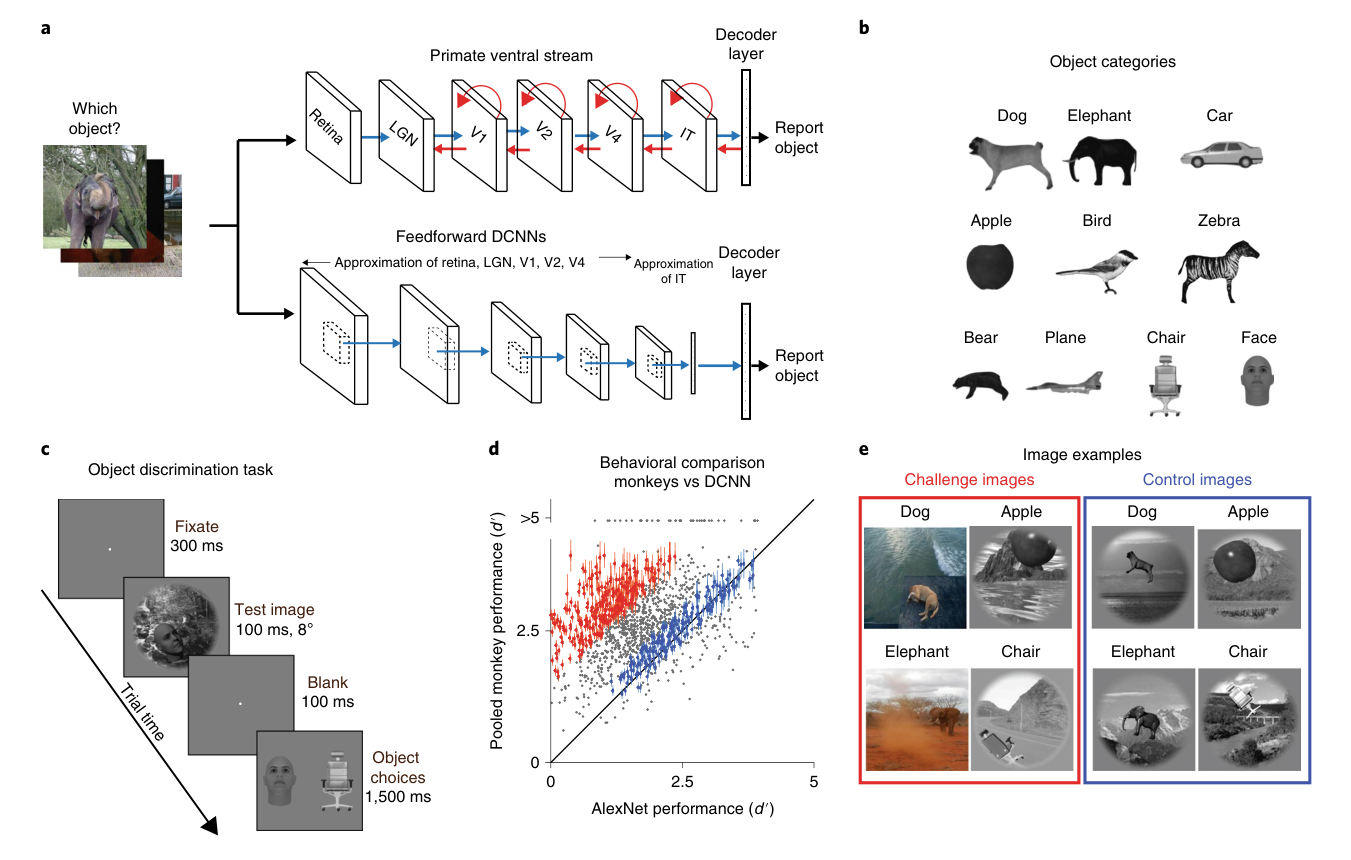
图 2 · IT 群体解码与逐图像解出时间(OST)
原文图注:Fig. 2 | Large-scale multiunit array recordings in the macaque IT cortex. a Schematic of array placement, neural data recording and OST estimation. We recorded extracellular voltage in the IT cortex (across the posterior, central and anterior inferior temporal cortices; PIT, CIT and AIT, respectively) from two monkeys, each hemisphere implanted with two or three Utah arrays. For each image presentation (100 ms), we counted multiunit spike events (see Methods for details), per site, in non-overlapping 10-ms windows, post stimulus onset, to construct a single population activity vector per time bin. These population vectors (image-evoked neural features) were then used to train and test cross-validated linear SVM decoders (d) separately per time bin. The decoder outputs per image (over time) were then used to perform a binary match to sample task and obtain NDAs at each time bin. An example of the neural decode accuracy over time is shown in the upper panel. The time at which the neural decodes equal the primate (monkey) performance is then recorded as the OST for that specific image. b, Examples of IT population decodes over time, with the estimated OSTs for four images: two control (top) and two challenge images (bottom). The red and blue circles represent the estimated neural decode accuracies at each time bins. The unbroken lines are nonlinear fits of the decoder accuracies over time (see Methods). The gray lines indicate the I1 performance of the primates (pooled monkey) for the specific images. Error bar indicates the bootstrapped s.e.m. c, Distribution of OSTs for control and challenge images. The median OSTs for control and challenge images are shown in the plot with broken lines. The inset on the top right shows the median evolution of IT decodes over time until the OST for control and challenge images.
读图要点:a 面板展示阵列覆盖 PIT/CIT/AIT 及分析流水线:每 10 ms 一个群体活动向量 → 每时间窗训练交叉检验线性 SVM → 与猴子行为水平(灰线,I1)比对确定 OST。b 面板给出四个例子:上方两张对照图像(文中示例 OST 分别约 135 和 122 ms),下方两张挑战图像(约 152 和 190 ms)——两组解码曲线都会爬升到猴子的行为准确率,但挑战图像到达该水平的时刻明显更晚。c 面板是两组 OST 的分布直方图,虚线标出中位数(对照约 115 ms,挑战约 145 ms),右上小图显示两组直到各自 OST 的解码准确率中位演化轨迹。这是全文的核心结果图,支撑上文结果 2。
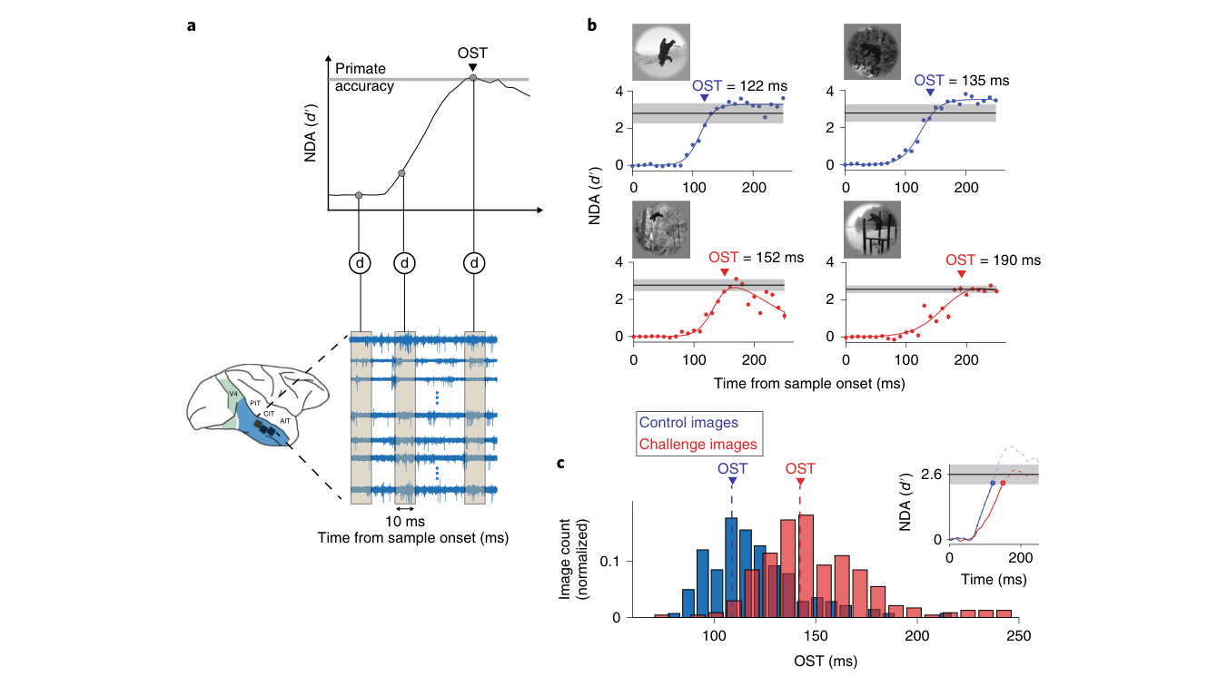
图 3 · 解出时间与神经响应潜伏期的关系
原文图注:Fig. 3 | Relationship between OSTs and neural response latencies. a Comparison of neural responses evoked by control (blue) and challenge (red) images. We estimated two measures of population response latency: population onset latency (tonset) and population peak latency (tpeak). b, Distributions of the population onset latencies (median across 424 sites), population peak response latencies (median across 424 sites) and OSTs for control images (n = 149). c, Same as in b but for challenge images (n = 266). d, Comparison of population onset latencies and OSTs for both control (blue; n = 149 images) and challenge images (red; n = 266 images). Vertical error bars show s.e.m. across neurons, and horizontal error bars show bootstrap (across trial repetition) standard deviations of OST estimates.
读图要点:a 面板把对照(蓝)与挑战(红)图像诱发的群体发放率曲线叠画在一起,并标出起始潜伏期(t_onset)与峰值潜伏期(t_peak)两个量;两组的起始时刻几乎重合,但挑战图像在约 150 ms 后的发放率更高。b、c 分别给出对照与挑战图像的 t_onset、t_peak 与 OST 三个分布:注意两种潜伏期都早于 OST,且两组的潜伏期分布几乎一样。d 面板是关键散点图:横轴为每张图像的群体起始潜伏期,纵轴为其 OST——蓝点(对照)与红点(挑战)形成两个几乎不重叠的水平层,而起始潜伏期与 OST 之间没有相关(r = 0.009),说明"解出更慢"与"响应更慢"是两回事。此图支撑上文结果 3 中排除视觉驱动变慢的论证。
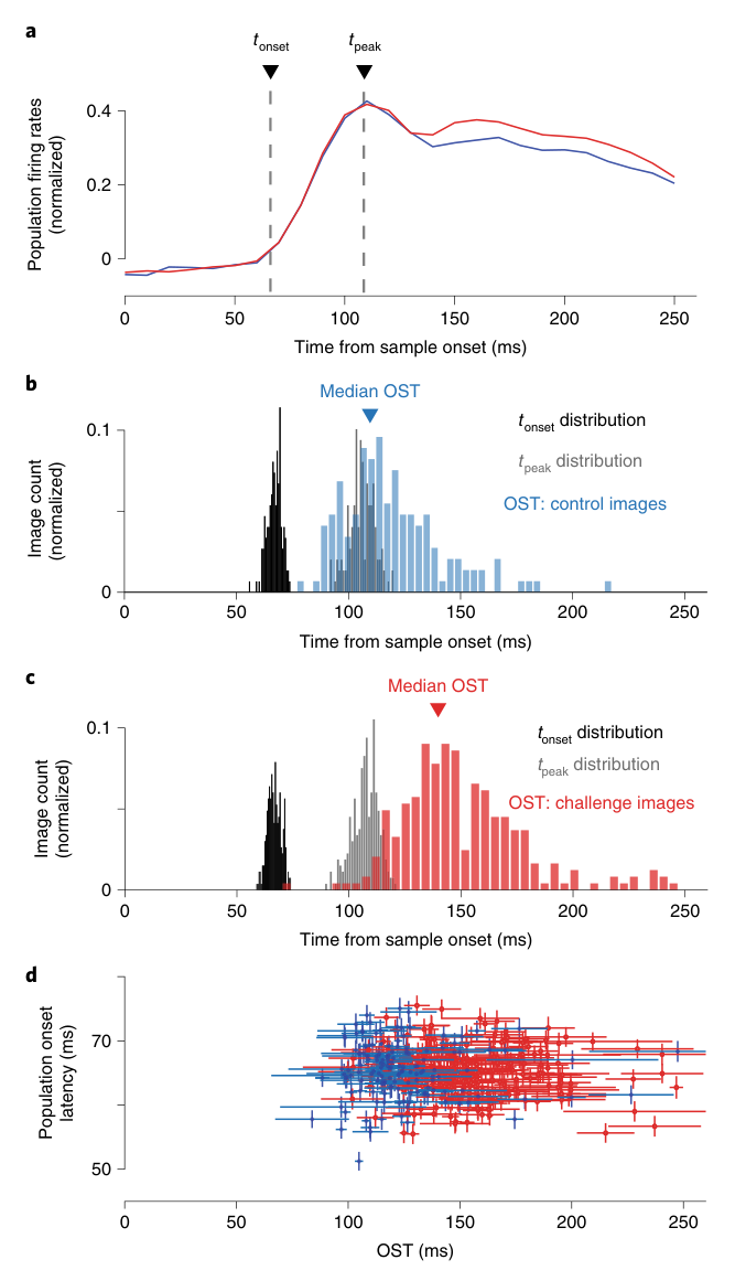
图 4 · 前馈模型对晚期 IT 响应预测失灵,更深与循环模型更好
原文图注:Fig. 4 | Predicting IT neural responses with DCNN features. a, IT predictivity of AlexNet's fc7 layer as a function of OST. For each time bin, we considered IT predictivity only for images that have a solution time equal to or higher than that time bin. Error bars indicate s.e.m. across neurons (n = 424 neurons considered for each time bin). Top: the distribution of OSTs for control (n = 149 images) and challenge (n = 266 images) images. b, IT predictivity computed separately for late OST images (OST > 150 ms, total of 349 images, n = 424 neurons) at the corresponding OSTs as a function of deep CNNs (AlexNet, Zeiler and Fergus, and VGG-S), deeper CNNs (Inception and ResNet) and deep-recurrent CNNs (CORnet). Circles indicate medians, and error bars indicate s.e.m. across neurons. Asterisks indicate a significant difference between two groups (obtained using paired t-tests). Deep (average of all three networks used) versus deeper CNNs (average of all four networks used): t(423) = 14.26, P < 0.0001. Deep (average of all three networks used) versus deep-recurrent (average of pass 3 and pass 4) CNNs: t(423) = 15.13, P < 0.0001. The inset to the right shows a schematic representation of CORnet that has recurrent connections (shown in red) at each layer (V1, V2, V4 and IT). For the boxplots, on each box, the central mark is the median, the edges of the box are the 25th and 75th percentiles, and the whiskers (W) extend to the most extreme data points that the algorithm considers not to be outliers. Outliers are data points that are larger than Q3 + W × (Q3 – Q1) or smaller than Q1 – W × (Q3 – Q1), where Q1 and Q3 are the 25th and 75th percentiles, respectively. Asterisk indicates a significant difference between two groups. c, Comparison of median OSTs for different sets of challenge images. The set of challenge images is defined with respect to each DCNN model. Thus, the exact set of images is different for each bar, the number of images is indicated on top of each bar, and the OST per image is plotted as a circle around each bar. In each case, the challenge images are defined as the set of images that remain unsolved by each model (using the fixed definitions of this study; see main text). Note that the use of deeper CNNs and the deep-recurrent CNN resulted in the discovery of challenge images that required even longer OSTs in the IT cortex than the original set challenge images (defined for AlexNet fc7).
读图要点:a 面板以时间为轴画 AlexNet fc7 的 IT predictivity:早期(约 90–110 ms)高达约 44%,随后随响应演化持续下滑,在 150–200 ms 段跌破 20%;上方小图叠加两组图像的 OST 分布,可以直观看到预测力下降的时段恰与挑战图像解出的时段重合。b 面板针对 OST > 150 ms 的 349 张图像,比较三类模型在其各自 OST 时刻的预测力:8 层"深"模型(AlexNet、Zeiler-Fergus、VGG-S)最低,>20 层的"更深"模型(Inception-v3/v4、ResNet-50/101)居中,带循环的 CORnet(取第 3、4 遍迭代)最高,星号标注配对 t 检验显著(深 vs 更深:t(423) = 14.26;深 vs 循环:t(423) = 15.13,均 P < 0.0001);右侧插图示意 CORnet 各层(V1/V2/V4/IT)都有红色循环连接。c 面板按"每个模型各自解不出的图像"重新定义挑战集,比较各集合的 OST 中位数(柱顶数字为图像数,如 AlexNet 266 张、CORnet 202 张等):模型越深(或带循环),其残余挑战图像的 OST 越长——即这些模型只部分地"预支"了循环计算。此图支撑上文结果 4。
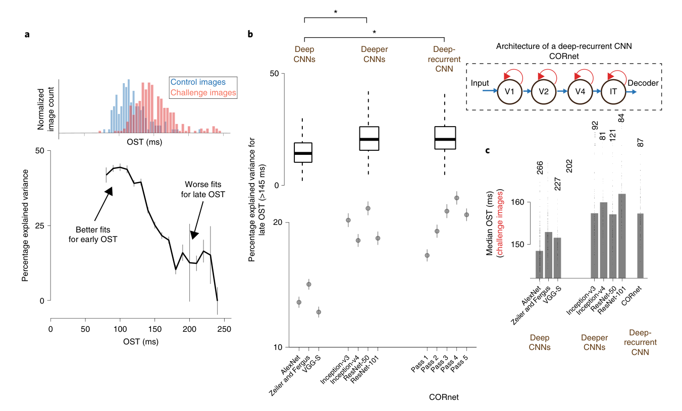
图 5 · 后向掩蔽对挑战图像的行为损伤更大
原文图注:Fig. 5 | Comparison of backward visual masking between challenge and control images. a, Binary object discrimination with backward visual masking. The test image (presented for 34, 67, 100, 134 or 267 ms) was followed immediately by a visual mask (phase-scrambled image) for 500 ms, followed by a blank gray screen for 100 ms, and then the object choice screen. Monkeys reported the target object by fixating it on the choice screen. b, Difference in behavioral performance between control and challenge images after backward visual masking. Each bar on the plot (y axis) is the difference in the pooled monkey performance during the visual masking task between the control and challenge images at the respective sample image presentation durations (x axis). The broken black line denotes the difference in performance between the control and challenge images without backward masking at the 100-ms presentation; n = 10 objects considered per presentation duration. Each circle corresponds to the difference in performance per object. The upper panel inset shows the raw performance (d') for the two groups of images. Error bars denote s.e.m. across all objects.
读图要点:a 面板给出掩蔽版任务时间线:测试图像分别呈现 34、67、100、134 或 267 ms 后立即接 500 ms 相位打乱的掩蔽图像,再空屏 100 ms 后进入选择屏。掩蔽被此前文献认为能选择性地切断某个脑区的再入式(循环)输入,使视觉加工停留在初始前馈响应上。b 面板的纵轴是"对照 − 挑战"的掩蔽任务表现差(正值即掩蔽对挑战图像伤害更大),横轴为呈现时长,黑色虚线标出无掩蔽时 100 ms 呈现下的基线差异;短呈现时长下各柱显著为正,267 ms 处差异归零。结合电生理结果,这构成"晚期 IT 响应对挑战图像的行为成功是必要的"这一行为层面的收敛证据,支撑上文结果 5。
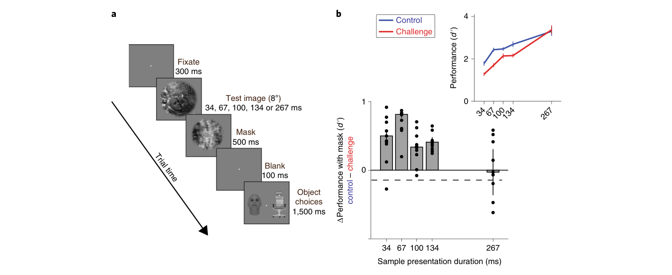
图 6 · 预测"循环参与":图像属性不如 Δd′ 向量
原文图注:Fig. 6 | Comparison of OST prediction strength. Comparisons were made between different image properties, a combination of all estimated image properties, and the Δd' vector (deviation of model behavior from pooled monkey behavior). Different image properties (n = 64 total: 32 high, 32 low; refer to Methods) for each image group was used. The red broken line denotes the significance threshold of the F-statistic. Image properties such as object size, eccentricity, presence of an occluder and a combination of these properties (referred to as All factors) significantly predict OST. However, the Δd' vector provided the strongest OST predictions. Error bars denote bootstrap standard deviations over images. The asterisk denotes a significant difference between the two groups, image properties versus Δd', estimated with repeated measures ANOVA (F(1,10) > 100, P < 0.0001; multiple-comparison using Turkey test showed a significant difference between Δd' and all other image properties). For the boxplot, on each box, the central mark is the median, the edges of the box are the 25th and 75th percentiles, and the whiskers extend to the most extreme data points that the algorithm considers not to be outliers. Outliers are defined as in Fig. 4b.
读图要点:这是一张箱线图,纵轴为各因素对 OST 的预测强度(单向 ANOVA 的 F 统计量,单位任意),横轴依次列出尺寸、偏心度、遮挡、杂乱、模糊、对比度、三种旋转等单一图像属性、"All factors"组合以及 Δd′ 向量;红色虚线为 F 统计量的显著性阈值。要点有二:尺寸、偏心度、遮挡及所有因素组合都能显著预测 OST,但都只是"踩线"的弱预测;而 Δd′(模型行为与猴子行为之差)的预测强度远超其他所有因素(重复测量 ANOVA F(1,10) > 100,P < 0.0001,Tukey 检验逐一确认)。此图支撑上文结果 6,也为讨论中"用图像可计算模型代替名词化图像属性"的主张提供数据。
讨论
作者的最简解释是:刺激诱发的 IT 响应晚期相依赖循环计算,且这些 IT 动态并非附带现象——掩蔽实验与行为对照表明它们对核心识别行为是关键的。至于这些循环回路住在哪,作者给出了一组可检验的猜想:以 V1 到 IT 之间每级约 10–15 ms 的传递节律计,约 30 ms 的额外时间相当于至少两个额外的加工阶段,因此既可能是 IT 与 V4/V2/V1 之间的皮层间反馈通路,也可能是来自前额叶与围嗅皮层的下游自上而下信号,还不能排除 IT 内部循环或皮层下回路(如基底神经节环路)——这些假设并不互斥。作者的贡献在于把宽泛的"反馈"概念收窄为一个实验上可操作、且保证行为相关的具体情形,并提出用靶向扰动实验逐个压制这些回路结构,而本研究给出的逐图像 OST 向量正好可以预测哪些图像最受扰动影响。作者也承认,Δd′ 虽是比单一图像属性好得多的实验指南,却仍未说明循环回路究竟解决了什么计算问题;他们推测循环计算相当于对初始前馈 IT 响应再做额外非线性变换,使其更线性可分——这与"有限时间循环网络可等价为带权重共享的极深前馈网络"的理论结果相呼应,即计算机视觉界靠堆层数达到的,大脑用循环架构更高效地实现了。最后,文章把三组交付物留给下一代模型:Δd′ 行为向量、逐图像 OST 向量、以及各图像在各自 OST 时刻的 IT 响应(目标特征),并指出固定的固定时间窗积分解码模型将因此面临被推翻的压力。
一句话总结
在我看来,这篇文章真正立住的不只是"反馈参与视觉识别"这句老话,而是一套把循环计算变成可测量、可证伪对象的操作体系:挑战图像是探针,OST 是读数,模型预测力随时间的衰减是交叉验证。它的局限也很清楚——"更深的 CNN 也能拟合晚期响应"恰恰说明行为证据还不足以把"循环"与"任意额外非线性变换"区分开,扰动实验才是终审。
审校与证据追溯 (Verification & Evidence)
图表审计结果
- Fig1: 提取质量
good,对齐度full,识别面板[] - Fig2: 提取质量
good,对齐度full,识别面板[] - Fig3: 提取质量
good,对齐度full,识别面板[] - Fig4: 提取质量
good,对齐度full,识别面板[] - Fig5: 提取质量
good,对齐度full,识别面板[] - Fig6: 提取质量
good,对齐度full,识别面板[]
关键事实与局限性声明
- 审校纠偏: OVERCLAIM(轻度,见 ISSUE_002):结果 5 标题将行为掩蔽证据表述为对晚期 IT 响应必要性的『证明』,超出原文 converging evidence 的定位;属作者推论被表述为已证事实。
- 审校纠偏: 注:解读讨论段与一句话总结对『更深 CNN 也能拟合晚期响应说明尚不能区分循环与任意额外非线性变换、扰动实验才是终审』的批判性评价属于审稿人自己的合理推断(INTERPRETATION),且以『在我看来』明确标示,不构成事实错误;该立场与原文作者自己承认的局限(需直接扰动实验)一致。
- 补充要点: 未提及端到端微调(fine-tuned)AlexNet 的稳健性检验:原文 Methods/Supplementary Fig. 14 显示三大主结果(挑战图像发现、滞后解出、晚期 predictivity 下降)在微调后的网络上依然复现,这是对『模型未见过训练集』质疑的重要对照。
- 补充要点: 未提及为平衡行为水平而丢弃 d' ≥ 5 的挑战图像(其平均 OST 为 150.2 ms,仍在挑战图像范围内)这一分析细节;该步骤排除『挑战图像只是行为更容易』的混淆,值得一提。
- 补充要点: 被动观看条件的结果只给了 ΔOST ≈ 28 ms,未提该条件下挑战图像晚期发放率同样更高(ΔR = 13.2%, t(423) = 8.27, P < 0.0001)及主动-被动 OST 相关 ρ = 0.76 已提及——前者可补。
- 补充要点: 未受训猴子分析中『未训练动物 IT 解码准确率整体小幅但显著下降(median Δd' = 0.23, t(639) = 7.78, P < 0.0001)』这一伴随负结果未提及。