IT Literature Intelligence 终审版本 (VERIFIED) 论文编号:
075| 原始基线:V0_ZCODE_BASELINE| 语义审核:needs_revision| 图表审核:pass
Learning Invariant Object and Spatial View Representations in the Brain Using Slow Unsupervised Learning
Rolls · Frontiers in Computational Neuroscience · 2021 · Zotero itemID=870
一句话定位:这篇综述是 Rolls 四十年来"不变表征如何被学习出来"这条研究线的总更新:从猕猴下颞叶(inferior temporal visual cortex, IT)与海马的空间视角(spatial view)细胞之神经生理证据出发,用自建的 VisNet 模型论证一个核心命题——大脑靠"利用环境统计规律的慢速无监督学习(slow unsupervised learning)"来学到对位置、尺寸、视角、形变乃至光照都不变的目标表征。它与深度学习的"教师信号 + 反向传播"路线形成鲜明对照,对关心生物合理性建模的读者是必读文献。
研究背景
问题域是视觉认知里最经典的一个:视网膜上的图像随目标的位置、尺寸、视角、光照与形变而剧烈变化,但大脑最终形成的面孔与目标表征却能跨这些变换保持不变(transform-invariant representations)。神经生理一侧当时已经积累了大量现象学证据:Rolls 团队自 1979 年起在下颞叶皮层和杏仁核记录到对面孔选择性放电的细胞,其不变性覆盖平移、尺寸与对比度、光照、空间频率乃至部分细胞的视角变换;这些细胞以稀疏分布式编码(sparse distributed coding)表征不同面孔,对以正确空间排列组合的特征敏感,且群体中分别存在调谐面孔身份、表情、头身运动的细胞。计算一侧的缺口在于机制:这些不变表征是怎么学出来的?彼时主流的人工智能方案是深度卷积网络——用上千个样本、以反向传播(backpropagation of error)配合"教师"逐神经元强制标注类别来训练。Rolls 认为这条路线在生物学上站不住:大脑突触是局部的,没有反向传播误差的通道,也没有逐神经元的教师,因此需要另寻机制。
第二条背景线索来自空间认知。啮齿类海马以位置细胞(place cells)著称,但 Rolls 团队在猕猴海马发现许多神经元编码的是"猴子正看向世界中的哪个方位"——空间视角细胞(spatial view cells),其表征对眼位、头朝向与个体所在位置均保持不变,甚至能在黑暗中由自我运动(idiothetic, self-motion)信号短暂更新。怎么让一个视觉系统学到这种对眼位、头向、所在位置三重不变的空间表征,是平移不变目标识别问题的空间版镜像,同样缺少统一机制解释。
研究思路
作者的总策略是"现象学先于机制、机制再回到现象学":先盘点 IT 皮层与海马细胞已知的反应性质,把这些性质当作模型的约束清单(例如自然场景中 IT 细胞感受野会收缩、识别只需前馈处理即可完成、新异目标首见时反应会被修改等),然后提出一个生物上可实现的计算模型来复现这些性质。核心概念是慢速学习:真实世界里同一目标的各个变换通常在时间上紧密相邻(连续注视间目标只发生小变换),于是可以在突触修改规则里引入一个短时记忆痕迹(trace)——让突触后活动的痕迹保持约 100 毫秒以上——使时间上相邻的输入被联系为"同一目标的不同变换"。这个思路最早由 Földiák(1991)针对平移不变性提出,Rolls 把它推广到所有类型的不变性,并落实进一个四级层级网络 VisNet。
推广的第二步是回答"这套原则有多通用"。作者让同一架构吃不同的输入与统计规律:把 Gabor 输入换成局部光流就得到背侧通路的全局运动表征;把时间连续性换成空间连续性就得到连续空间变换学习(continuous spatial transformation, CT learning);把增益调制(gain modulation)与痕迹学习结合就得到背侧系统到顶叶的坐标变换链。全文的论证骨架正是"一个学习原则、多个脑系统复用"——这也被作者明确表述为一种皮层运算原理的再利用。
方法
VisNet 是四级前馈层级竞争网络(competitive network),模仿腹侧视觉通路:Layer 1 对应 V2,Layer 4 对应前部 IT(TE),各层 32×32 个神经元,每神经元接受来自上一层高斯分布连接半径内约 200 个突触(Layer 1 为 272 个;教程版可扩到每层 256×256 神经元、1000 突触),层间感受野约按 2.5 倍逐级放大,使第四层能覆盖整个"视网膜"输入(Fig. 1)。改为“输入由模拟 V1 的 Gabor 滤波器提供,包括4个空间频率、4个朝向和正负两种极性,共32个滤波通道。”每层内的"竞争"通过稀疏度参数实现:激活先按突触权重做点积,再经阈值线性或 Sigmoid 函数转成放电率,阈值设定使该层表征稀疏度 a 约为 0.01(稀疏度按跨神经元的归一化定义给出)。
学习规则是全文的方法核心:第 2–4 层用带痕迹的联想式突触修改,δwj = α·ȳτ·xj,其中痕迹 ȳτ = (1−η)yτ + η·ȳτ−1,η 通常取 0.8;Layer 1 则用纯联想规则(无痕迹),以保证特征的空间相对位置在不变性学习开始前就被正确绑定(解决特征绑定问题)。训练时同一目标的所有变换以随机顺序连续呈现,再换下一个目标。生物学实现上,作者主张痕迹可由 NMDA 受体的长时间常数或局部吸引子网络(attractor network)维持——IT 细胞在刺激消失后常继续放电约 1 秒,且逆向掩蔽实验表明识别可只由前馈完成,这些都被引为支持。改为“本文引用了 VisNet 与 HMAX 的直接模型比较;对 HCNN 则主要进行概念性和生物合理性讨论,并未报告统一基准下的头对头测试。”空间部分使用 VisNetCT 模型(Rolls, 2020),把增益调制与痕迹学习结合逐级做坐标变换。
主要结果
-
不变表征的神经生理清单(第一部分证据)。IT 面孔/目标细胞的平移、尺寸、对比度、光照、空间频率、视角不变性在文中被逐一引证;在复杂自然场景中它们的感受野从空白背景下的约 70° 直径收缩到约 8° 半径(对 5° 刺激),使视觉系统每次只处理中央凹附近的目标,多目标的位置靠中央凹与旁中央凹反应的不对称性编码(Aggelopoulos 与 Rolls 的五目标实验);新异目标在最初几次呈现时反应被修改而熟悉目标不受影响,被解读为颞叶皮层自组织构建新表征的证据。海马一侧,空间视角细胞编码的是外部中心(allocentric)坐标中"看向哪里",对眼位、头朝向与所在位置不变(Rolls et al., 1997a, 1998; Georges-François 等 1999),且在黑暗与帘幕遮挡下仍能被自我运动更新几分钟,之后随路径积分记忆的消耗而漂移(Robertson 等 1998)。
-
VisNet 学会各类变换不变性,且不是查找表。特征绑定先行的设计得到验证:四种线条的全部组合可以各自形成独立表征(Elliffe 等 2002);中间层的特征组合神经元可被更高层复用为多个不同目标的组件(Rolls and Mills, 2018,Fig. 2),这是高容量的关键。训练后的网络在杂乱背景与部分遮挡下识别几乎不受损(Stringer and Rolls, 2000),训练序列中混入其他目标也不妨碍不变性学习(Stringer and Rolls, 2008)。
-
同样的架构、不同的输入统计 → 不同的表征类型。旗帜形变实验(Webb and Rolls, 2014,Fig. 3)显示:同一网络若在时间上相近地看到同一姿态/形变的不同个体,就学出姿态特异、对个体与视角不变的表征;若在时间上相近地看到同一个体的不同姿态/形变,就学出身份特异、对姿态与形变不变的表征——功能架构完全相同,只改时间统计就能换一种被学到的表征。非意外性质(non-accidental properties, NAP,如凹缘 vs 凸缘 vs 直缘)实验(Rolls and Mills, 2018,Fig. 4)进一步表明:痕迹规则让"随视角连续变化的度量性质"(曲率程度)被泛化掉,而"跨视角不变的非意外性质"被保留——与真实物体的自然统计行为一致。
-
与 HMAX、HCNN 的对照实验。两只杯子各 4 个视角(Fig. 7):VisNet 学到 100% 正确的视角不变表征——第四层自组织出只对"Bill"或只对"Jane"全部视角放电的神经元;HMAX 则完全分不开两个物体,反而对带文字的图像反应更强,说明它更像一组图像滤波器。HMAX 末层神经元调谐很差、表征过于分布,与 IT 皮层不符;VisNet 和 IT 神经元一样不对打乱五官的 scrambled 面孔反应,而 HMAX 对打乱与否照单全收——差异正来自 VisNet 用时间连续性学到了"哪些图像属于同一目标"。容量方面:教程版 VisNet 在 50 个真实世界目标、每目标 9 个间隔 40° 的视角上训练后,任意视角识别 90% 正确(随机水平 2%),对离最近训练视角 20° 的插值视角为 68% 正确。作者对 HCNN 的批评是方法论层面的:先训练到神经元相似再宣称"这就是大脑的计算方式"存在循环论证,何况反向传播与卷积权重复制都是非局部、非生物的运算。
-
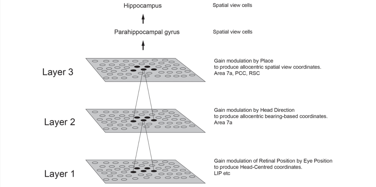
背侧系统复用同一套原则。全局运动方面,把 V1 输入换成局部光流后,同一 VisNet 架构在第三层产生位置不变的全局运动神经元(Fig. 9)——两个轮子在不同位置旋转,局部小感受野无法判定旋转方向,层级汇聚加痕迹学习解决了这个问题;模型还复现了 Hasselmo 等(1989b)发现的目标中心运动表征(如头部顺时针转动,与正立/倒置无关)。空间坐标变换方面(Fig. 10):视网膜坐标经眼位增益调制变为头中心的自我中心表征(LIP/VIP),再经头朝向调制变为"指向地标的方位"表征(顶叶 7a、后扣带),最后经个体位置调制变为外部中心空间视角表征——每级增益调制都叠加痕迹慢速学习,改为“在 VisNetCT 模拟中,慢速学习降低了多级坐标变换中不精确性的累积;作者据此提出,该通路可能向海马空间视角细胞提供短时遮挡期间的自我运动更新信号。”此外慢速学习还被延伸到海马形成机制:竞争学习把内嗅皮层网格细胞映射为齿状回/CA1 位置细胞,痕迹规则能解释位置野较宽以及障碍物处位置野中断的现象(Muller and Kubie, 1987)。
图注解读
图 1 · 视觉系统的逐级汇聚与 VisNet 架构对应
原文图注:FIGURE 1 | Convergence in the visual system. (Right) Convergence in the ventral stream cortical hierarchy for object recognition. LGN, lateral geniculate nucleus; V1, visual cortex area V1; TEO, posterior inferior temporal cortex; TE, anterior inferior temporal cortex (IT). (Left) Convergence as implemented in VisNet, the model of invariant visual object recognition described here. Convergence through the hierarchical feedforward network is designed to provide Layer 4 neurons with information from across the entire input retina, by providing an increase of receptive field size of 2.5 times at each stage. Layer 1 of the VisNet model corresponds to V2 in the brain, and Layer 4 to the anterior inferior temporal visual cortex (TE). In this paper 'Layer' with a capital L indicates a Layer of a neuronal network which may correspond to a brain region as here. This is distinct from the 6 architectonic layers in neocortex, designated here with a small letter l in 'layer'.
这张图左右并置:右侧是真实腹侧通路的层级(LGN→V1→TEO→TE),左侧是 VisNet 的四层实现。读图的关键是"汇聚"(convergence)这个概念——每级感受野扩大 2.5 倍,使第四层神经元能汇总来自整个视网膜的信息;同时给出了明确的映射约定:VisNet Layer 1 ≈ V2,Layer 4 ≈ 前部 IT(TE),大写 Layer 指网络层、小写 layer 指新皮层六层构造,避免混淆。它支撑方法部分的架构设定,也是全文"为什么只需要 4–5 层"这一论断的图示来源——层级汇聚本身就是一种计算,不必堆上百层。
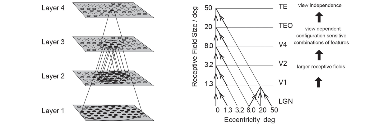
图 2 · 中间层特征组合神经元的复用
原文图注:FIGURE 2 | Encoding of information in intermediate Layers of VisNet. The 13 stimuli used to investigate independent coding of different feature combinations by different neurons in intermediate Layers of VisNet. Each of the 13 stimuli was a different feature, or feature combination with adjacent features, that was learned to be a different object by VisNet, demonstrating that VisNet can learn to represent objects as different even when they have overlapping features. Moreover, these feature combination neurons could be used by further combination in higher Layers of VisNet to represented more complex objects. (After Rolls and Mills, 2018).
图中是 13 个由简单线条特征(及其与相邻特征的组合)构成的刺激。读法:VisNet 把 13 个刺激学成 13 个不同的"目标",尽管它们共享部分特征——这证明中间层学到的是特征组合的独立编码而非把特征打散。这些组合神经元随后可在更高层被再次组合成更复杂目标,即"组件复用"。这张图支撑结果第 2 条中"VisNet 不是查找表"的论断:正因为中间表征是可复用的组件,末层才能以高容量表征大量目标,也让早期层学到的自然特征能加速新目标的学习。
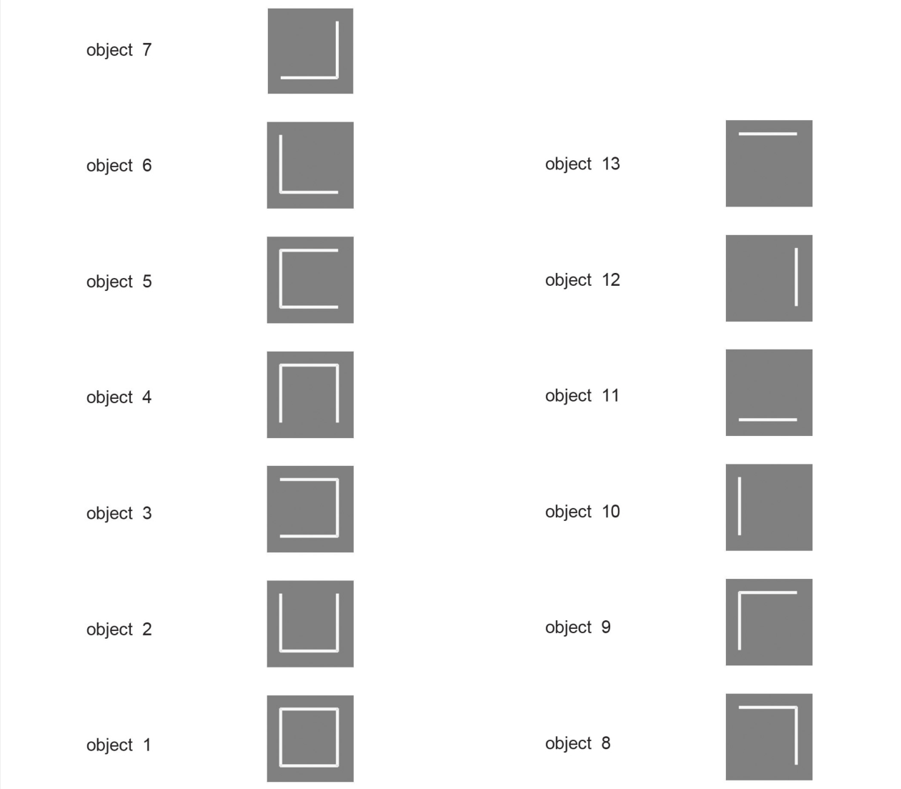
图 3 · 形变不变识别的旗帜刺激
原文图注:FIGURE 3 | Deformation-invariant object recognition. The flag stimuli used to train VisNet to demonstrate deformation-invariant object recognition. Each flag is shown with different wind forces and rotations. Starting on the left with the first pair of images for each flag, both the 0 and 180°views are shown for a windspeed of 0; and each successive pair is shown for the wind force increased by 50 Blender units. Visnet learned to categorize these 4 flags as 4 different flags provided that the different deformations of each flag were shown close together in the temporal sequence during training, to make use of the trace learning rule. (After Webb and Rolls, 2014).
四个旗帜目标,各自展示 0° 与 180° 两个视角,风力从 0 开始逐对增加 50 个 Blender 单位,因此同一旗帜的图像形态被风力拉得很开。读图要点是训练方式而非刺激本身:只有当每面旗帜的不同形变在训练序列中时间上紧密相邻时,VisNet 才能把它们归类为同一旗帜——这正是痕迹规则起作用的条件。这张图支撑结果第 3 条"形变不变表征"的来源,也形象化了"环境统计决定学到什么"的原则。
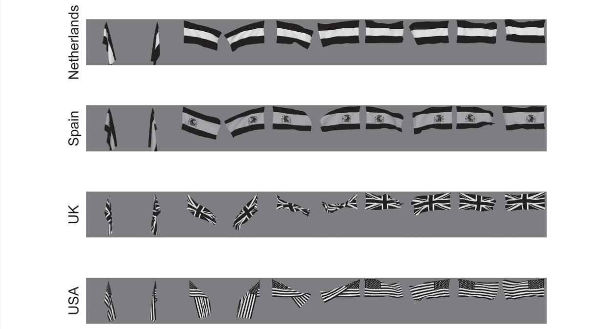
图 4 · 非意外性质与度量性质的分离
原文图注:FIGURE 4 | Learning non-accidental properties of objects. The stimuli used to investigate non-accidental properties (NAP) vs. metric properties (MP) of encoding in VisNet. Each object is shown as white on a gray background. Objects 1–3 all have the non-accidental property of concave edges. Objects 1–3 are different in their metric properties, the amount of curvature. Object 4 has the non-accidental property of parallel edges. Objects 5–7 have the non-accidental property of convex edges, and different metric properties from each other, the amount of the convexity. The vertical view of each object was at 0°of tilt, with the images at –6 and 6°of tilt illustrated. Different amounts of tilt of the top toward or away from the viewer are shown at the tilt angles indicated. Each object was thin, and was cut off near at the top and bottom of each object to ensure that any view of the top or bottom of the object did not appear, so that the type of curvature of the edges (concave, straight, or convex) was the main cue available.
七个细长物体分三组:1–3 为凹缘(曲率度不同)、4 为平行缘、5–7 为凸缘(凸出度不同)。刺激被上下截断、只在 −6°/0°/6° 倾角间变化,保证边缘曲率类型是唯一可用线索。读图关键在"哪些差异跨视角保持、哪些随视角连续变化":NAP(凹/凸/直/平行)不变,MP(曲率程度)连续变。结果 VisNet 对度量差异泛化、对非意外差异保持敏感——即痕迹规则自动把"跨时间稳定的东西"学成不变性质。这张图支撑结果第 3 条的后半部分。
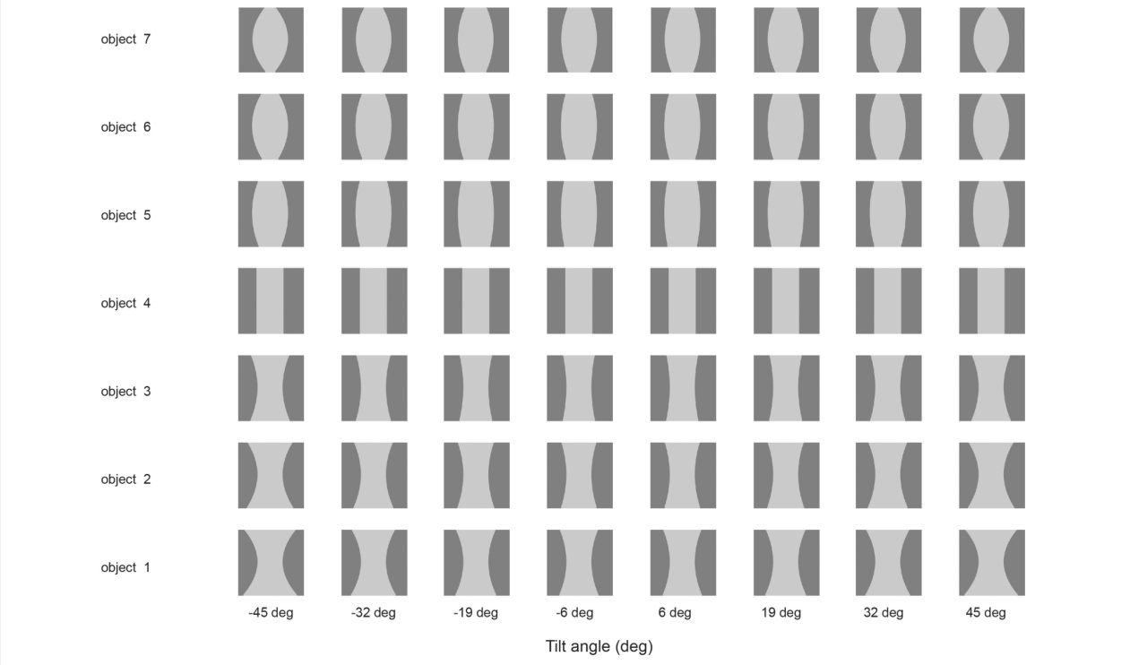
图 5 · 层级化 + 注意调控的皮层架构模型
原文图注:FIGURE 5 | Cortical architecture for hierarchical and attention-based visual perception. The system has six modules organized so that they resemble the ventral visual stream (Left) and dorsal visual stream (Right) of the primate visual system. Information from the lateral geniculate (LGN) enters V1. The ventral visual stream leads through V2–V4 to the inferior temporal visual cortex (IT), and is mainly concerned with object recognition. The dorsal visual stream leads via areas such as MT into the posterior parietal cortex (PP), and is involved in this model in maintaining a spatial map of an object's location. The solid lines with arrows between levels show the forward connections, and the dashed lines the top-down backprojections. Short-term memory systems in the prefrontal cortex (PF46) apply top-down attentional bias to the object (from PFv) or spatial processing (from OFd) streams. (After Deco and Rolls, 2004).
六个模块按腹侧(LGN→V1→V2–V4→IT,管"是什么")与背侧(经 MT→后顶叶 PP,管"在哪里")双流组织,实线为前馈、虚线为自上而下反投影,前额叶短时记忆系统(PFv 面向目标、OFd 面向空间)施加注意偏置。这张图的用法是给"注意在自然场景中的作用"提供架构背景:在该架构下模型复现了 IT 神经元在复杂场景中感受野收缩、自上而下注意在朴素背景下对反应的调制更强等现象(Deco and Rolls, 2004)。它支撑的是方法与讨论中"自然场景里中央凹占优"的机制解释(Fig. 5 所示的皮层放大率与竞争),属于背景性架构图。
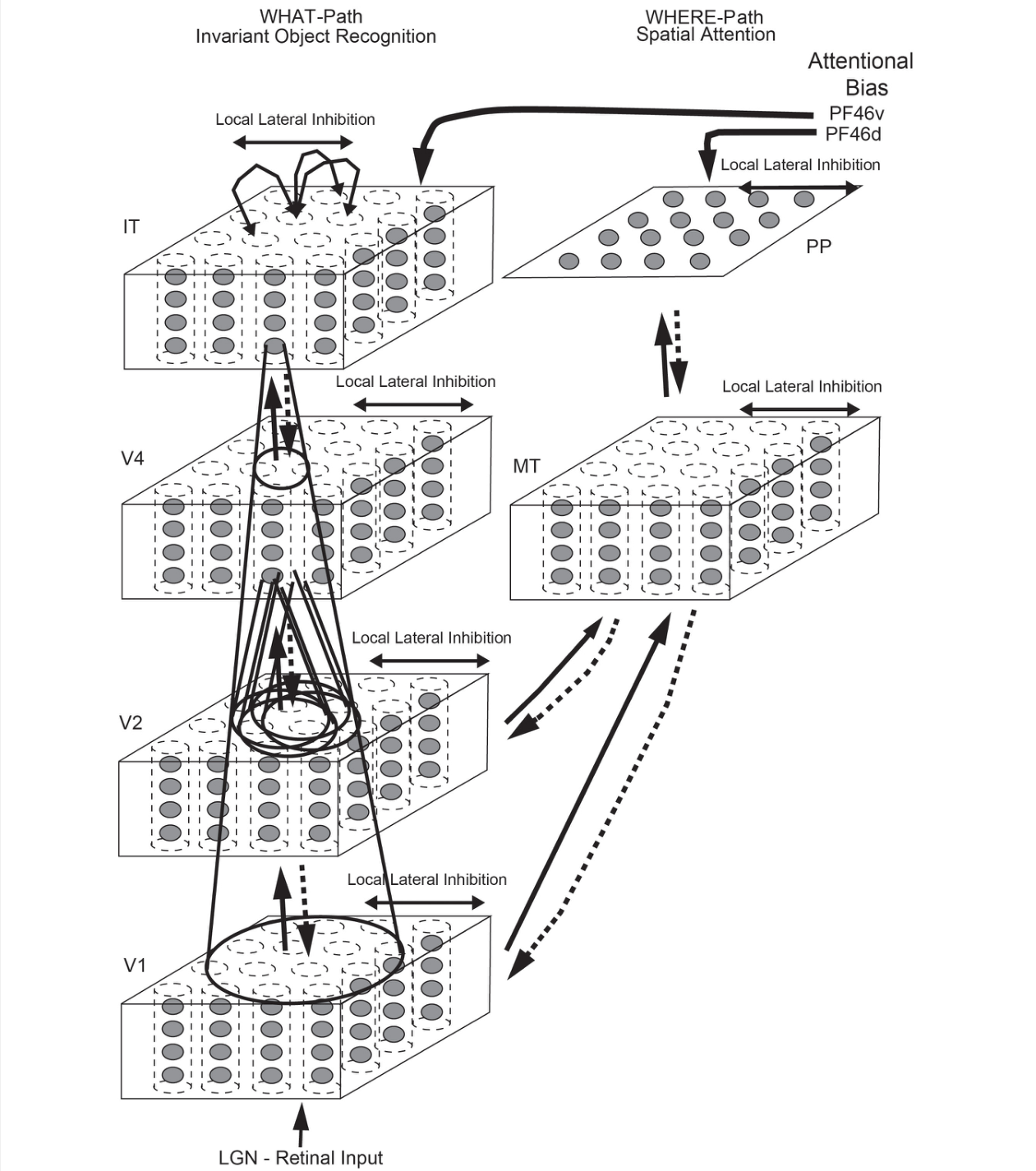
图 6 · 自然场景中找目标与认目标的联合仿真
原文图注:FIGURE 6 | Finding and recognizing objects in natural scenes. (A) Eight of the twelve test scenes. Each scene has four objects, each shown in one of its 4 views. (B) The bottom-up saliency map generated by the GBVS code for one of the scenes. The highest levels in the saliency map are red, and the lowest blue. (C) Rectangles (384 pixels × 384 pixels) placed around each saliency peak in the scene for which the bottom-up saliency map is illustrated in (B). (After Rolls and Webb, 2014).
三联图:A 是 12 幅测试场景中的 8 幅,每幅含 4 个目标(各取 4 个视角之一);B 是对其中一幅用 GBVS(graph-based visual saliency)生成的自下而上显著性图(红=高,蓝=低);C 是在每个显著性峰上放置的 384×384 像素矩形,作为"注视"窗口喂给 VisNet。读法是跟着流水线走:背侧系统算显著性 → 引导"眼动"到显著位置 → 腹侧系统对注视矩形内的内容做不变识别。性能为 90% 正确(随机 25%),且不依赖目标是否恰在注视中心,还能泛化到训练视角(相隔 45°)之间的中间视角。这张图支撑结果第 4 条之前提——腹侧系统需要同时实现约 8° 的平移不变性与视角不变性,因为显著性引导的眼睛很少正好落在目标中心。
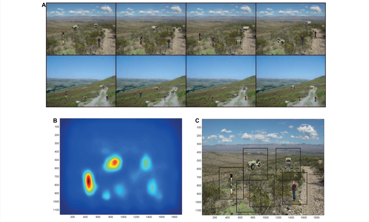
图 7 · 杯子实验:VisNet 能而 HMAX 不能
原文图注:FIGURE 7 | View invariant representations by VisNet but not by HMAX. The two objects, cups, each with four views. HMAX of Riesenhuber and Poggio (1999) fails to categorize these objects correctly, because, unlike VisNet, it has no slow learning mechanism to associate together different views of the same object. (After Robinson and Rolls, 2015).
两只杯子、各 4 个视角。这张图是 HMAX 与 VisNet 正面对比的实验材料:两个目标从某些视角看图像性质差异不大、且不同目标之间共享低层特征(包括杯上的文字),按"图像特征分类"的逻辑几乎不可分。结果 VisNet 100% 正确分出两杯(第四层自组织出各对一杯全部视角放电的神经元),HMAX 则按文字有无反应、完全分不开。读图要抓住"视角不变必须靠学"这一点:HMAX 的 S-C 层级没有任何机制把"同一目标的不同视角"联系在一起,VisNet 靠时间连续性 + 痕迹规则做到了。这张图支撑结果第 4 条,也是全文对"无慢速学习的特征层级走不远"的最直观演示。
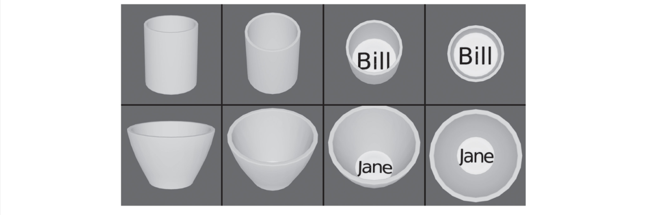
图 8 · 连续空间变换(CT)学习原理
原文图注:FIGURE 8 | Continuous spatial transformation learning of transform-invariant visual representations of objects. This illustrates how continuous spatial transformation (CT) learning would operate in a network with forward synaptic connections between an input Layer of neurons and an output Layer. Initially the forward synaptic connection weights are set to random values. (A) The presentation of a stimulus to the network in position 1. Activation from the active (shaded black) input neurons is transmitted through the initially random forward connections to activate the neurons in the output Layer. The neuron shaded black in the output Layer wins the competition in the output Layer. The synaptic weights from the active input neurons to the active output neuron are then strengthened using an associative synaptic learning rule. (B) The situation after the stimulus is shifted by a small amount to a new partially overlapping position 2. Because some of the active input neurons are the same as those that were active when the stimulus was presented in position 1, the same output neuron is driven by these previously strengthened synaptic afferents to win the competition. The rightmost input neuron shown in black is activated by the stimulus in position 2, and was inactive when the stimulus was in position 1, now has its synaptic connection to the active output neuron strengthened (denoted by the dashed line). Thus the same neuron in the output Layer has learned to respond to the two input patterns that have vector elements that overlap. The process can be continued for subsequent shifts, provided that a sufficient proportion of input neurons is activated by each new shift to activate the same output neuron. (After Stringer et al., 2006).
示意图分两拍:A 中刺激在位置 1 呈现,竞争获胜的输出神经元把来自活跃输入神经元的突触加强;B 中刺激小幅移动到部分重叠的位置 2,由于部分输入神经元相同,先前加强过的传入使同一个输出神经元再次获胜,新激活的输入(虚线)也被连到它——于是同一个输出细胞学会响应所有空间上逐渐平移的输入模式。读图要点是"空间重叠"替代了"时间痕迹"作为联系的来源,因此 CT 学习不需要时间连续性、甚至允许与其他目标交错训练;代价是训练中的变换必须在空间上足够接近。这张图支撑结果第 3 条中空间连续性路线的原理说明。
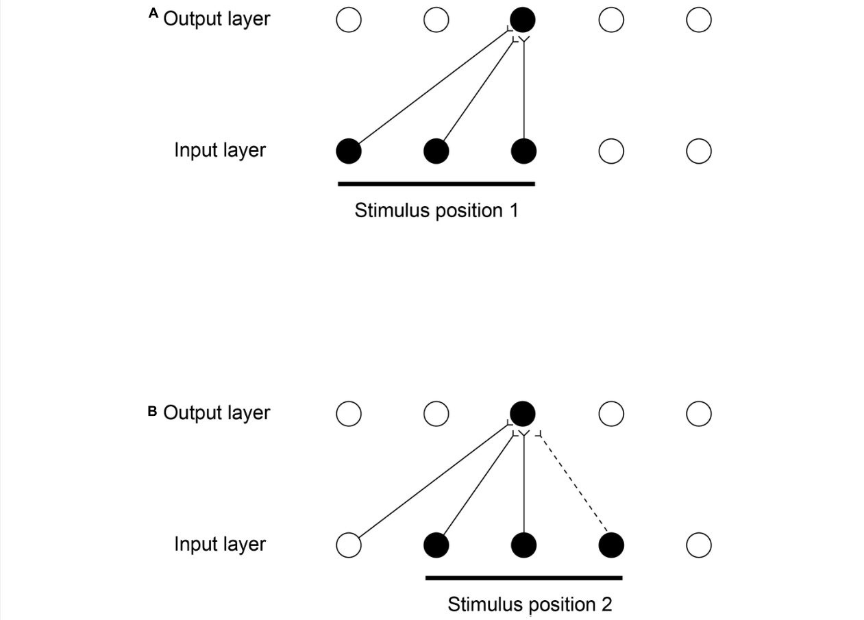
图 9 · 背侧系统的位置不变全局运动
原文图注:FIGURE 9 | Invariant object-based global motion in the dorsal visual system. This shows two wheels at different locations in the visual field rotating in the same direction. One rotating wheel is presented at a time, and a representation is needed in the case illustrated that the rotating flow field produced by the wheel in either location is always clockwise. The local flow field in V1 and V2 is ambiguous about the direction of rotation of the two wheels, because of the small receptive field size. Rotation that is clockwise or counterclockwise is can only be identified by a global flow computation, with larger receptive fields. The diagram shows how a network with stages like those found in the brain can solve the problem to produce position invariant global motion-sensitive neurons by Layer 3. The computation involved is convergence from stage to stage as illustrated, combined with a short-term memory trace synaptic learning rule to help the network learn that it is the same wheel rotating in the same direction as it moves across the visual field during training (during development). This is the computational architecture of VisNet. It was demonstrated that VisNet can learn translation invariant representations of these types of object-based motion, by substituting the normal Gabor filters as the input neurons in the input Layer corresponding to V1 with local optic flow motion neurons also present in V1. (After Rolls and Stringer, 2006b).
图中两个轮子出现在视野不同位置、旋转方向相同(顺时针)。计算困境在于:V1/V2 的局部光流感受野太小,无法判定整体旋转方向,只有更大感受野的全局流计算才能区分顺/逆时针。网络解法与 VisNet 同构——逐级汇聚 + 短时记忆痕迹规则(训练时同一轮子移动着穿过视野、方向不变),到第三层就产生位置不变的全局运动神经元。读图时注意方法细节:只需把输入层里模拟 V1 的 Gabor 滤波器换成 V1 中同样存在的局部光流运动神经元即可。这张图支撑结果第 5 条的背侧运动部分,并例证"同一皮层运算原理在不同脑区复用"。
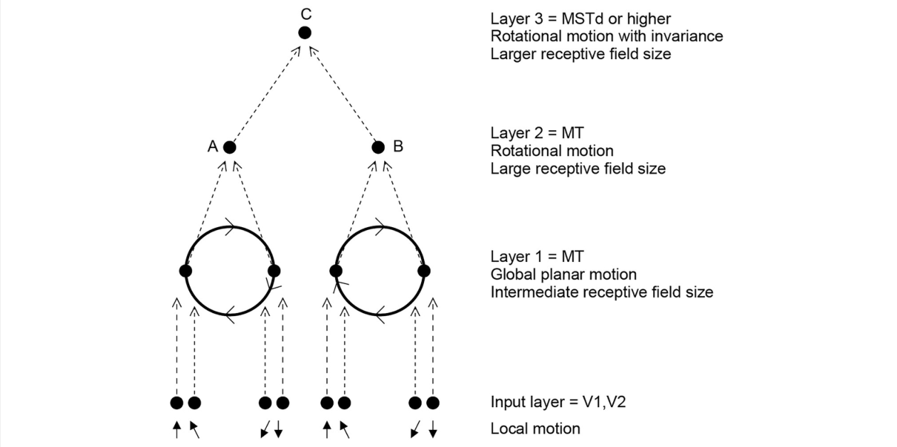
图 10 · 三级坐标变换:从视网膜坐标到海马空间视角
原文图注:FIGURE 10 | Coordinate transforms in the primate dorsal visual system. Three stages of coordinate transforms that take place at different levels of the primate dorsal visual system are shown. At each stage the coordinate transform is performed by gain modulation of the receptive field by an appropriate modulator, that is usefully combined with slow learning of the type implemented in VisNet which helps the same neurons at a particular stage to develop what are effectively representations that become independent of the modulating signal. In Layer 1 gain modulation by eye position combined with slow learning enables neurons to develop representations in head-centered coordinates that are invariant with respect to retinal and eye position. In Layer 2 gain modulation by head direction combined with slow learning enables neurons to develop representations in allocentric bearing to a stimulus such as a landmark coordinates that are invariant with respect to head direction. In Layer 3 gain modulation by the place where the individual is located combined with slow learning enables neurons to develop representations of a stimulus such as a landmark that are in allocentric spatial view coordinates with invariance with respect to where the individual is located. The diagram shows the architecture of the VisNetCT model in which gain modulation combined with short-term memory trace associative learning was shown to implement these transforms (Rolls, 2020). Each neuron in a Layer (or cortical area in the hierarchy) receives from neurons in a small region of the preceding Layer. It is proposed that idiothetic update through this dorsal visual cortical stream is used for idiothetic update of hippocampal spatial view cells useful for navigation when the environment may not be visible for short periods (Rolls, 2020, 2021b). PCC, posterior cingulate cortex; RSC, retrosplenial cortex.
这张图是空间部分的支柱图:三级变换链——Layer 1 用眼位增益调制把视网膜坐标变为头中心坐标,Layer 2 用头朝向调制变为"指向地标的方位"(外部中心),Layer 3 用个体所在位置调制变为纯外部中心的空间视角坐标(经顶叶、压后皮层 RSC 与后扣带 PCC 通往海马系统)。每级的组合式都是"增益调制 + 痕迹慢速学习":前者提供瞬时变换,后者把同一空间位置在不同调制条件下的输入绑定到同一组神经元,使表征逐步摆脱调制信号本身。读图时顺着三层往右看不变性如何逐级累加,再联系正文:这正是海马空间视角细胞能在视野被短暂遮挡时靠自我运动(idiothetic)更新继续导航的机制来源。该图支撑结果第 5 条的空间部分。
讨论
讨论部分有两块内容。第一块是把模型细节与皮层解剖对应起来:沿腹侧流从 V1 到 TE,第三层锥体细胞基树突覆盖面积、树突长度、棘密度与侧支连接范围都逐级增大,基树突棘数从 V1 的约 640 个增至 TE 的约 7400 个——作者将其解读为功能分工的证据:早期阶段必须保持高空间分辨率以精确绑定特征(T 还是 L),因此 Layer 1 只用纯联想规则、不引入不变性;而高层阶段需要大感受野覆盖目标的所有变换,且痕迹学习需要由侧支连接实现的局部吸引子网络把活动维持一秒上下(IT 细胞在刺激撤除后放电常持续约 1 秒、可被逆向掩蔽打断,正支持这一主动维持机制)。第二块是与深度学习的对照及对人工智能的启示:卷积深度网络依赖非局部的反向传播与权重复制、需要逐输出神经元的教师,训练上用海量单帧样本"暴力"拟合,缺少系统性的同一目标变换集,因此学到的是像素级表征(改几个像素就能失效,也对对抗样本敏感)。作者据此建议:用同一目标的变换序列训练人工网络,能更有效地学到变换不变的形状表征。
局限方面,作者坦率承认两点:其一,VisNet 能否按比例放大到解释灵长类(包括人类)的目标识别尚难断言——文中给出的容量数字来自教程版实现,真实新皮层每个模块约十万神经元、每个锥体细胞约两万突触(约一万给侧支、五千给前馈、五千给止于第一层的反投影),腹侧系统可能有数十到数百个这样的模块,稀释连接有助于容量,但缩放问题没有定论;其二,把侧支吸引子用来做变换不变识别的替代方案因视角数 s 的巨大代价(O = kC/s)而未被继续推进,吸引子更可能用于"清理"歧义图像成类别。与文献的对话贯穿全文:从 Földiák 的痕迹规则与慢特征分析(slow feature analysis, Wiskott & Sejnowski 2002)一脉的后续工作,到 Hasselmo 的目标中心运动细胞、啮齿类位置/网格细胞系统,再到 Yamins 与 DiCarlo 的 HCNN 匹配路线。关于物种差异作者还补了一句值得注意的话:啮齿类没有中央凹、眼动控制的背侧系统与后扣带皮层也不发达,可能更多依赖基于位置的导航,而灵长类(包括人类)的空间视角细胞提供了一条不需欧氏几何计算、逐地标导航的更简路径。
一句话总结
我读这篇综述的感受是:Rolls 在做的事情与其说是"提出一个模型",不如说是把"环境的时间—空间统计规律 + 局部突触可塑性"立为大脑自组织的一条第一性原理,然后改为“作者用目标识别、形变、全局运动和坐标变换的既往模拟与神经生理现象,论证这一原则可能具有跨系统适用性,但其脑内因果机制仍待直接检验。”要提醒读者的是,文中对深度学习的批评带有明显的立场(反向传播"生物不合理"的争论远未终结),VisNet 的缩放能力也确是软肋;但"同一目标的不同变换在时间上扎堆出现,本身就携带了不变性的答案"这个洞察,我认为是任何认真思考视觉学习的人都绕不开的。
审校与证据追溯 (Verification & Evidence)
图表审计结果
- Fig1: 提取质量
good,对齐度full,识别面板[] - Fig10: 提取质量
good,对齐度full,识别面板[] - Fig2: 提取质量
good,对齐度full,识别面板[] - Fig3: 提取质量
good,对齐度full,识别面板[] - Fig4: 提取质量
good,对齐度full,识别面板[] - Fig5: 提取质量
good,对齐度full,识别面板[] - Fig6: 提取质量
good,对齐度full,识别面板[A, B, C] - Fig7: 提取质量
good,对齐度full,识别面板[] - Fig8: 提取质量
good,对齐度full,识别面板[A] - Fig9: 提取质量
good,对齐度full,识别面板[]
关键事实与局限性声明
- 审校纠偏: {'classification': 'INTERPRETATION', 'statement': 'HCNN 与脑神经元相似属于循环论证。', 'assessment': '这是 Rolls 对相关建模路线的批评性解释,不是本文通过新数据确立的事实;V0 后文虽提示其立场性,但方法和结果部分仍应明确归因于作者。'} -> 评注: 这是 Rolls 对相关建模路线的批评性解释,不是本文通过新数据确立的事实;V0 后文虽提示其立场性,但方法和结果部分仍应明确归因于作者。
- 审校纠偏: {'classification': 'OVERCLAIM', 'statement': 'VisNetCT 的结果证明了背侧通路驱动海马空间视角细胞更新并支持导航。', 'assessment': '模型只证明该计算方案可行并改善模拟性能;实际脑区通路及导航因果作用在本文中仍是提议。'} -> 评注: 模型只证明该计算方案可行并改善模拟性能;实际脑区通路及导航因果作用在本文中仍是提议。
- 审校纠偏: {'classification': 'OVERCLAIM', 'statement': '四类应用反复验证了慢速无监督学习作为普遍皮层运算原理。', 'assessment': '现有证据支持跨任务计算可行性和与若干神经现象的一致性,但不能确立该机制在真实脑内的普遍性、必要性或充分性。'} -> 评注: 现有证据支持跨任务计算可行性和与若干神经现象的一致性,但不能确立该机制在真实脑内的普遍性、必要性或充分性。
- 审校纠偏: {'classification': 'FACT', 'statement': 'VisNet 在两只杯子、各四个视角的特定测试中达到100%正确,而所测试的 HMAX 神经元未区分两个物体。', 'assessment': '该结果及方向在原文中明确存在,但适用范围限于 Robinson and Rolls(2015)的具体刺激、实现和评价设置,不应外推为所有 HMAX 或所有物体识别任务的普遍结论。'} -> 评注: 该结果及方向在原文中明确存在,但适用范围限于 Robinson and Rolls(2015)的具体刺激、实现和评价设置,不应外推为所有 HMAX 或所有物体识别任务的普遍结论。
- 补充要点: : (第 1 页)
- 补充要点: : (第 16 页)
- 补充要点: : (第 5 页)
- 补充要点: : (第 18 页)